An introduction to Momocs

News

As of Oct. 2018, Momocs is being extensively polished these days and may evolve before its 2.0 release as part of MomX.

Preliminaries

Abstract

Momocs aims to provide a complete and convenient toolkit for morphometrics. It is intended for scientists interested in describing quantitatively the shape, and its (co)variations, of the objects they study.

In the last decade, R has become the open-source lingua franca for statistics, and morphometrics known its so-called “revolution”. Nevertheless, morphometric analyses still have to be carried out using various software packages either dedicated to a particular morphometric and/or for which source code is mostly unavailable and/or copyrighted. Moreover, most of existing software packages cannot be extended and their bugs are hard to detect and thus correct. This situation is detrimental to morphometrics: time is wasted, analyses are restricted to available methods, and last but not least, are poorly reproducible. This impedes collaborative effort both in software development and in morphometric studies.

By gathering the common morphometric approaches in an open-source environment and welcoming contributions, Momocs is an attempt to solve this twofold problem.

Momocs hinges on the core functions published in the must-have Morphometrics with R by Julien Claude (2008), but has been further extended to allow other shape description systems. So far, configurations of landmarks, outlines and open outline analyses, along with some facilities for traditional morphometrics are implemented.

Prior to analysis, Momocs can be used to acquire and manipulate data or to import/export from/to other formats. Momocs also has the facility for a wide range of multivariate analyses and production of the companion graphics. Thus a researcher will find that just a few lines of code will provide initial results, but the methods implemented can be finely tuned and extended according to the user’s needs.

If you use it, please cite it: citation("Momocs").
This citation refers to an obsolete version of Momocs, only handling outline analyses. The next companion, encompassing all MomX and seminal paper is on its way.

Survival tips

This vignette introduces Momocs, as for every R function, each function has its own manual page, eg ?efourier.
There is a much nicer online version of this manual that can be accessed from the console with, e.g. Momocs_help("efourier").
Feel free to contribute to Momocs through GitHub: report issues, ask for new features, share data and methods, correct typos, write better vignettes, helpfiles, or whatever pleases you. If you have never heard of GitHub, that’s definitely worth a look.
Feel free to drop me a line, should you need a hand or would like to collaborate with me: bonhomme.vincent@gmail.com.
Before asking for help, please read Momocs’s FAQ: vignette("Momocs_FAQ").

Get, install and use it

First, of all, let’s download the last version of Momocs. You will need to install the devtools package - if you do not have it yet - to get it from my GitHub repository :

install.packages("devtools")
devtools::install_github("MomX/Momocs")

The typical install_packages("Momocs") will get you the last CRAN version of Momocs, but the GitHub version is preferred as Momocs is still under active development.

We can start using Momocs, as long as it has been loaded using:

library(Momocs)

Design

Keywords used all accross Momocs are introduced here in bold.

Morphometrics is the ugly job of turning beautiful shapes into quantitative variables. Just kidding, that’s pretty exciting.

A shape is defined as a collection of (x; y) coordinates. No 3D yet but different families are handled by Momocs:

outlines, here in a first-quarter moon ;
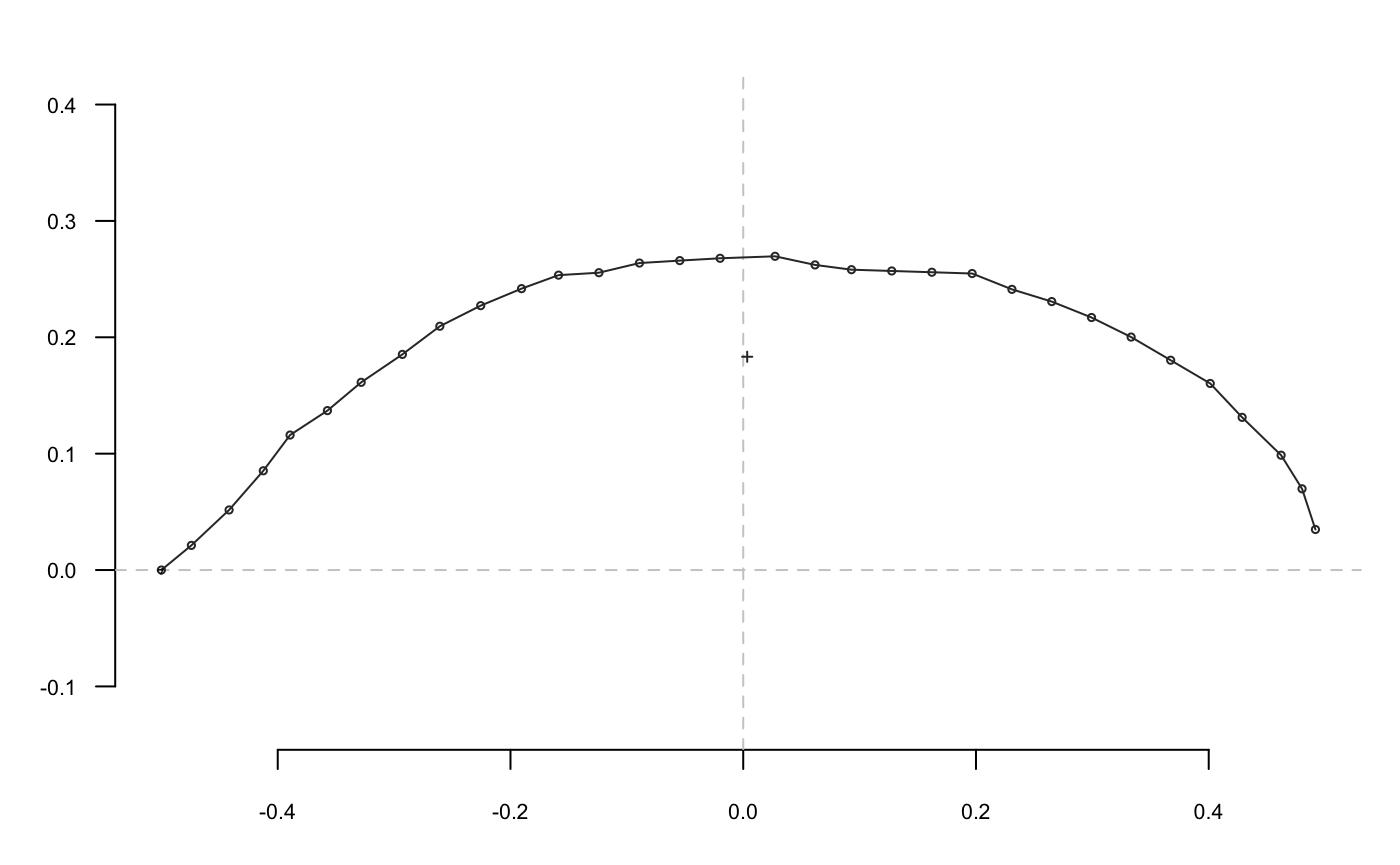
open outlines, here is the sterile valve of an olive stone;
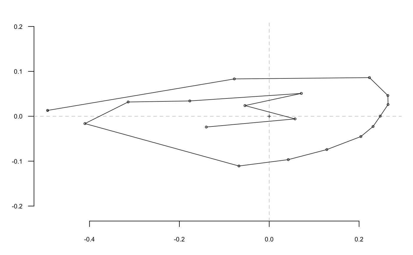
configuration of landmarks; here, homologous points from a mosquito wing.

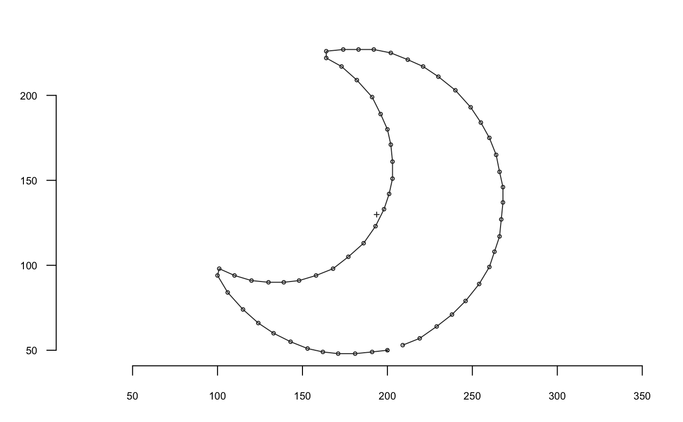
They are all single shapes defined by a matrix of (x; y) coordinates; here are the first points of the moon:

shapes[18] %>% head()

##      [,1] [,2]
## [1,]  200   50
## [2,]  199   49
## [3,]  198   49
## [4,]  197   50
## [5,]  196   50
## [6,]  195   49

Many operations on shapes are implemented such as: plotting, geometric operations, scalar descriptions, etc. These operations have their dedicated vignette, see vignette("Momocs_coo").

Working on single shape can quicly be boring. Shapes can be organized into a collection of coordinates: a Coo object that carries:

a component named $coo, a list of shapes (as matrix.ces);
most of the time, a component named $fac, a data.frame (or the modern equivalent, a data_frame) to store covariates, either factors or numerics;
possibly, other components of interest.

One can do several things with a Coo object: visualize it, apply morphometric operations, handle the data it contains, but in the end, a __ morphometric method__ will turn coordinates into coefficients.

Such morphometric operation on coordinates produce a collection of coefficients: a Coe object that carries:

a component named $coe, a matrix of coefficients;
if present in Coo, $fac is inherited;
possibly, other components of interest.

This can be summarized as follows:

`Coo`	+	Morphometric method	=	`Coe`
`(x; y)` coordinates	+	appropriate method	=	quantitative variables

Coo objects are collections of coordinates that become Coe objects when an appropriate morphometric method is applied on them.

Some operations on Coo/Coe are generic in that they do not depend of the nature of the shape. For instance, centering a configuration of landmarks or an outline, or calculating their centroid size is, mathematically, the same generic operation. But some operations on shapes are specific to a peculiar family. For instance, calculating elliptical Fourier transforms on a configuration of landmarks would make no sense.

Momocs implement this desirable behavior and defines classes and subclasses, as S3 objects.

`Coo`	Morphometrics methods	`Coe`
`OutCoo` (outlines)	`efourier`, `rfourier`, `sfourier`, `tfourier`	`OutCoe`
`OpnCoo` (open outlines)	`npoly`, `opoly`, `dfourier`	`OpnCoe`
`LdkCoo` (configuration of landmarks)	`fgProcrustes`, `slide`	`LdkCoe`

In other words:

any collection of shapes belongs to (pick one) {OutCoo, OpnCoo, LdkCoo} and is also a Coo object;
generic and specific methods can be applied to it
a collection of coefficients is obtain and belongs to (pick one) {OutCoe, OpnCoe, LdkCoe} and is also a Coe object.

Finally, generic and specific operations can be applied to the Coe objects, chiefly multivariate methods, capitalicized: PCA, LDA, CLUST, MANOVA(and MANCOVA), MSHAPES, KMEANS, etc.

Overall, Momocs implements a simple and consistent grammar that is detailed below. Also, if you’re familiar with modern R and the Hadley-verse, you should feel home as ggplot2 graphics, dplyr verbs and magrittr pipes are implemented.

Single shapes

Let’s load one of the Momocs datasets, some various outlines (an Out object):

shapes                    # prints a brief summary
panel(shapes, names=TRUE) # base graphics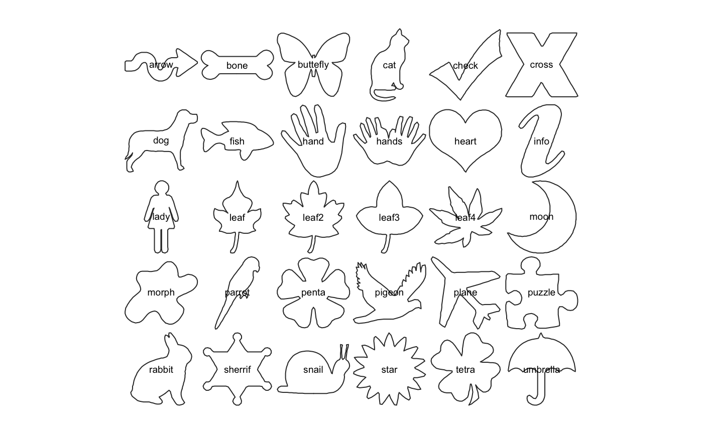

## Out (outlines)
##   - 30 outlines, 836 +/- 255 coords (in $coo)
##   - 0 classifiers (in $fac): 
## # A tibble: 0 x 0
##   - also: $ldk

shapes is one of the datasets bundled with Momocs. It’s (“lazy”) loaded in memory as soon as you call it, no need for data(shapes). To see all Momocs’ datasets, try data(package="Momocs"). These datasets are all Coo objects (try class(bot)), ie collection of shapes.

One can do many things on a Coo object, as above, eg printing a summary of it (just by typing its name in the console), plotting a family picture with panel, etc.

So far, we’re interested in single shapes so let’s extract the 4th shape from shapes, using the traditional syntax. We plot it with coo_plot that comes with several options for plotting all families of shapes.

shp <- shapes[4]
coo_plot(shp)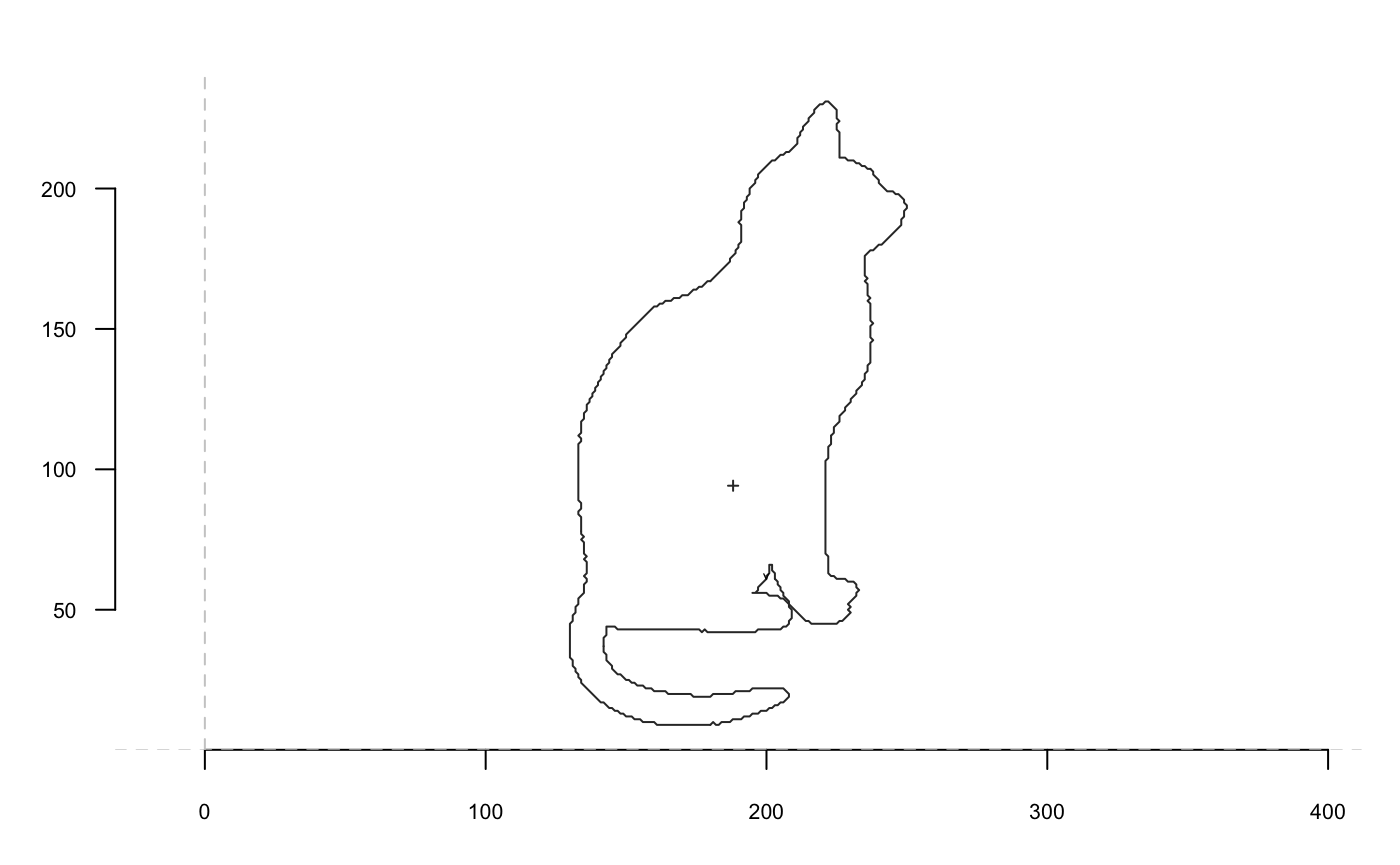

# coo_plot is the base plotter for shapes
# but it can be finely customized, see ?coo_plot
coo_plot(shp, col="grey80", border=NA, centroid=FALSE, main="Meow")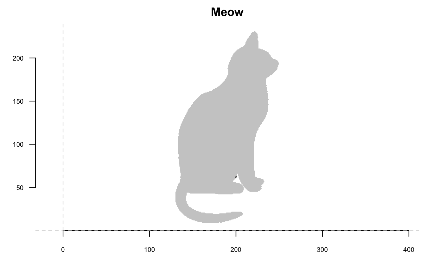

Let’s now do some basic operations on this shape. They all named coo_* and you can have the full list with apropos("coo_"). coo_* family encompasses:

geometric operations (such as centering, scaling, etc.)
plotting functions
scalar descriptors of shape (such as area, perimeter, circularity, rectilinearity, etc.)
various other operations on a single shape.

coo_plot(coo_center(shp), main="centered Meow")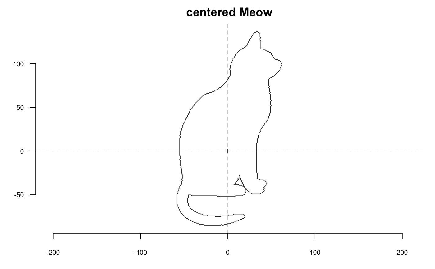

coo_plot(coo_sample(shp, 64), points=TRUE, pch=20, main="64-pts Meow")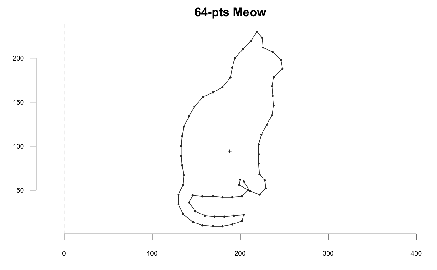

Momocs is fully compatible with maggritr’s pipe operators. A nice introduction can be found there. magrittr requires a (very small) cerebral gymnastics at the beginning but the benefits are huge, for defining moprhometric pipelines in Momocs but also for R as a whole. It makes things clearer, it: saves typing; reduces intermediate variable assignation; reads from left to right; substantiates the pipe we (should) have in mind. magrittr’s pipes are already loaded with Momocs.

shapes[4] %>% coo_smooth(5) %>% coo_sample(64) %>% coo_scale() %>% coo_plot()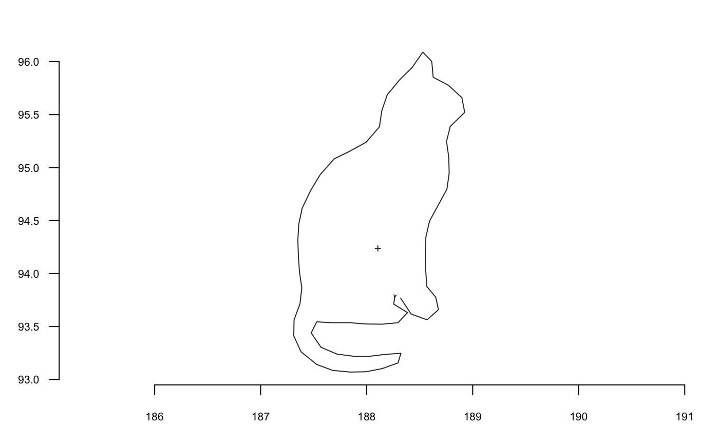

# pipes can be turned into custom function
cs64 <- function(x) x %>% coo_sample(64) %>% coo_scale() %>% coo_center()
shapes[4] %>% cs64 %>% coo_plot() # note the axes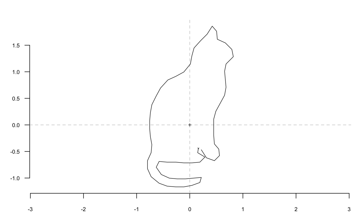

Have a look to the dedicated vignette with vignette("Momocs_coo").

The most familiar operation can directly be applied on Coo objects:

bot %>%
coo_center %>% coo_scale %>%
coo_alignxax() %>% coo_slidedirection("up") %T>%
print() %>% stack()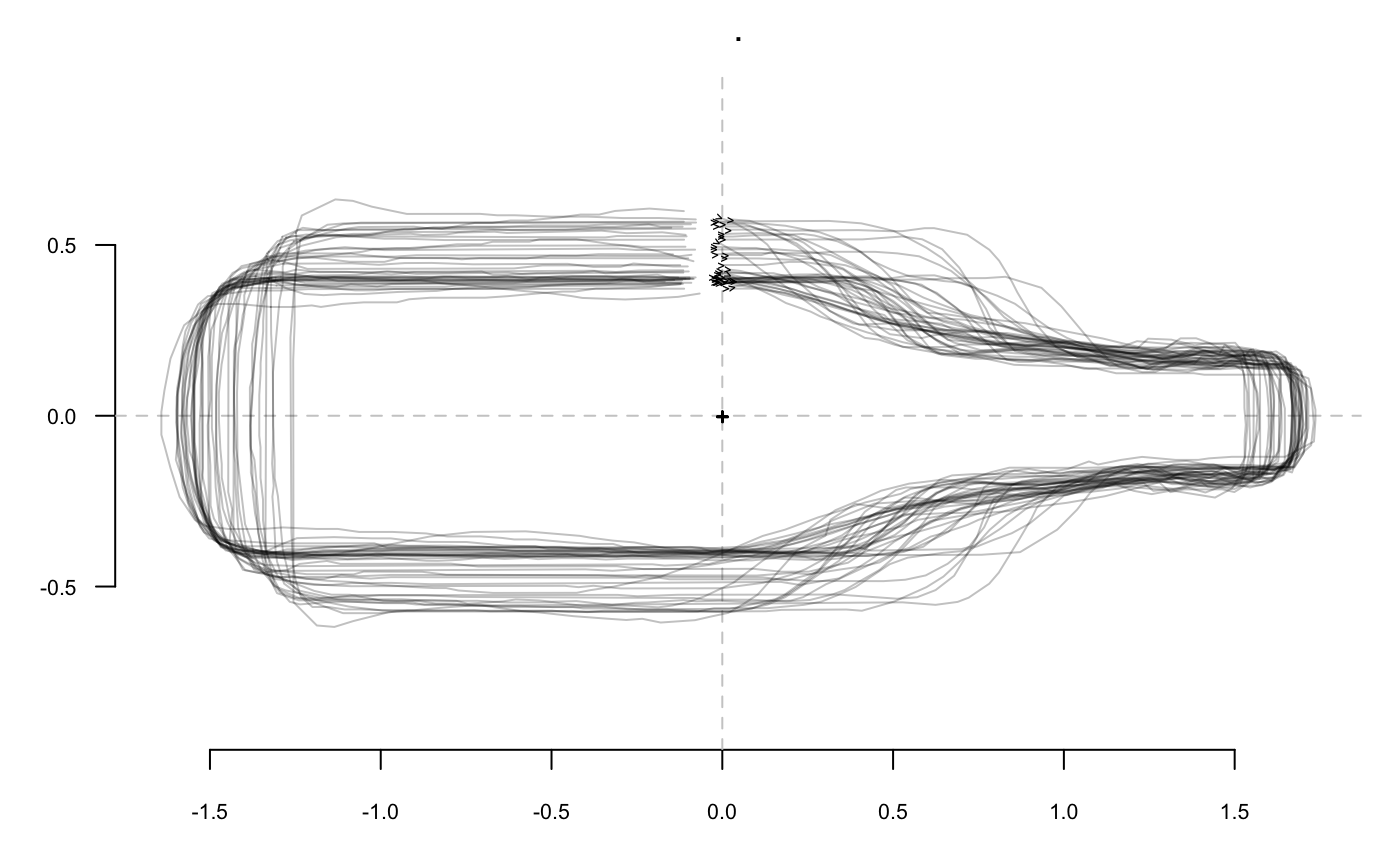

## Out (outlines)
##   - 40 outlines, 162 +/- 21 coords (in $coo)
##   - 2 classifiers (in $fac): 
## # A tibble: 40 x 2
##   type   fake 
##   <fct>  <fct>
## 1 whisky a    
## 2 whisky a    
## 3 whisky a    
## 4 whisky a    
## 5 whisky a    
## 6 whisky a    
## # ... with 34 more rows
##   - also: $ldk

Morphometrics

Outline analysis

A word about data import: you can extract outlines from a list of black masks over a white background, as .jpg images with import_jpg. Have a look to helpfiles (import_jpg and import_jpg1) for more details. Here we do not bother with import since we will use the bottles outlines dataset bundled with Momocs.

data(bot)
bot
panel(bot, fac="type", names=TRUE)

stack(bot)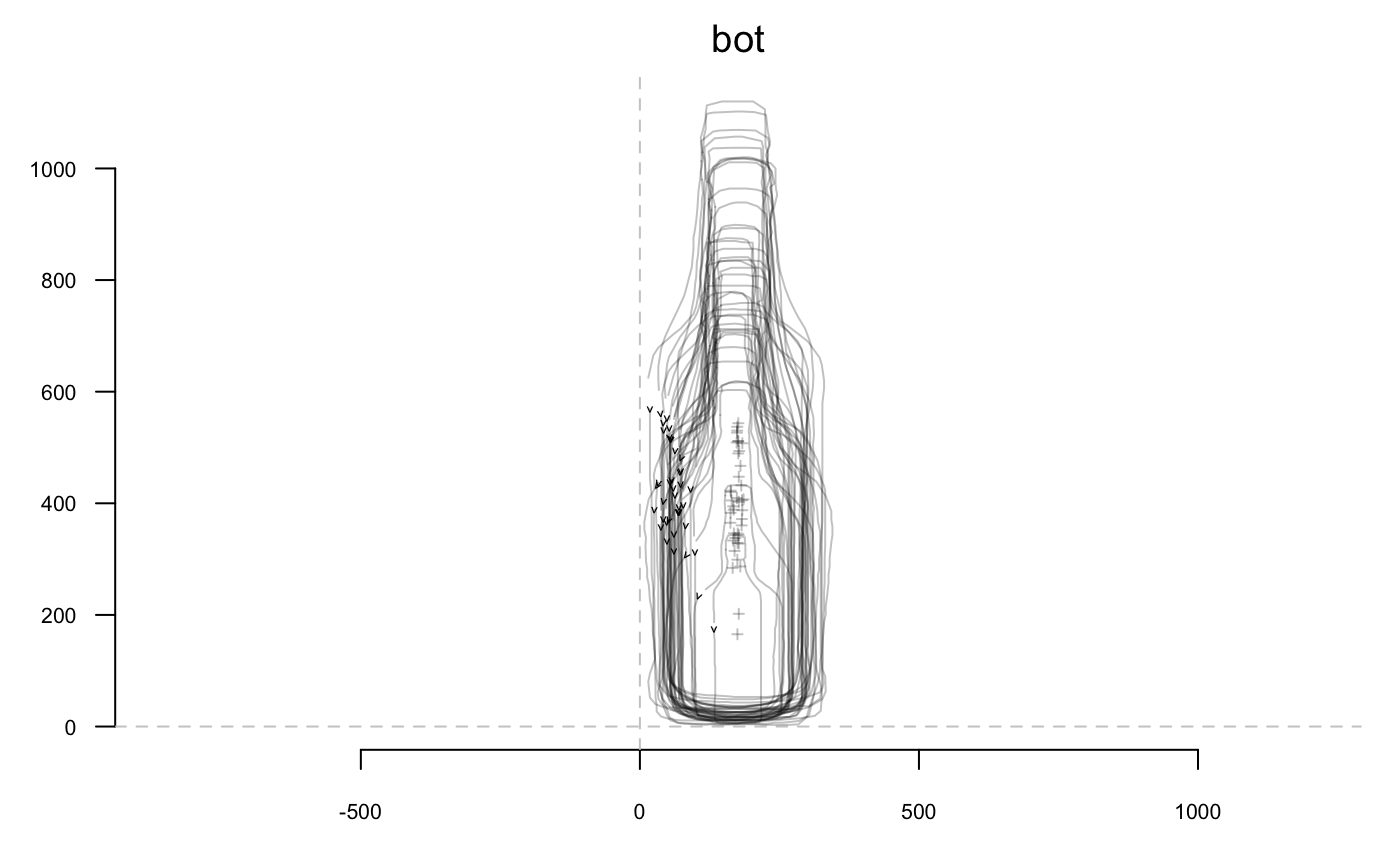

## Out (outlines)
##   - 40 outlines, 162 +/- 21 coords (in $coo)
##   - 2 classifiers (in $fac): 
## # A tibble: 40 x 2
##   type   fake 
##   <fct>  <fct>
## 1 whisky a    
## 2 whisky a    
## 3 whisky a    
## 4 whisky a    
## 5 whisky a    
## 6 whisky a    
## # ... with 34 more rows
##   - also: $ldk

Here, we will illustrate outline analysis with elliptical Fourier transforms (but the less used and tested rfourier, sfourier and tfourier are also implemented).

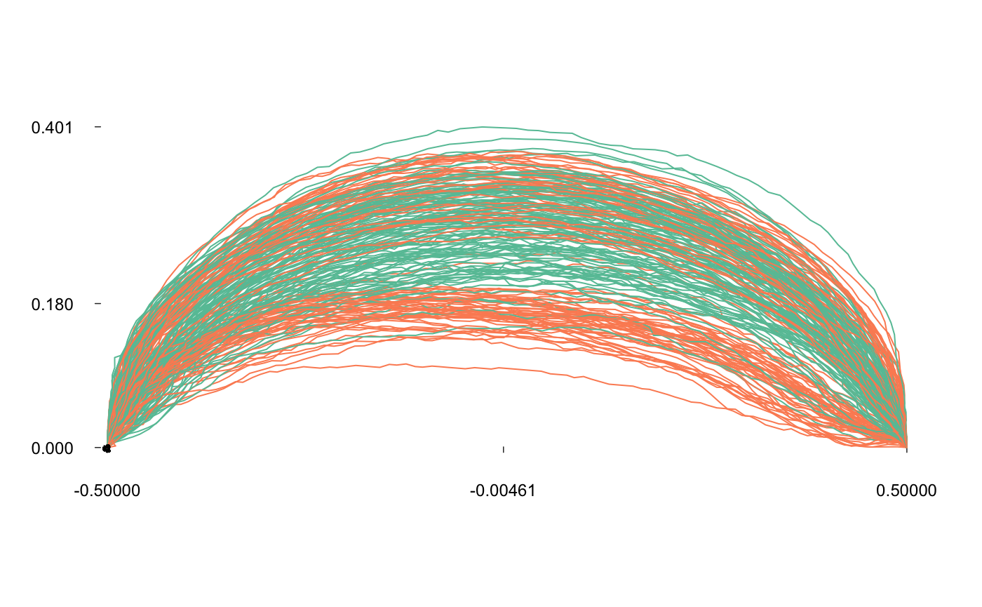
The idea behind elliptical Fourier transforms is to fit the x and y coordinates separately, that is the blue and red curves below:

coo_oscillo(bot[1], "efourier")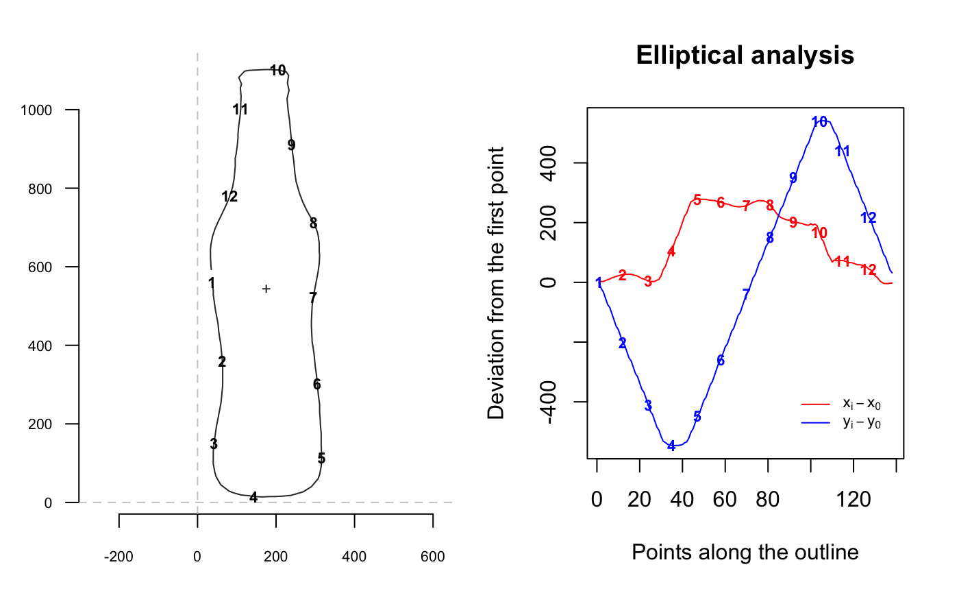

## # A tibble: 138 x 2
##       dx    dy
##    <dbl> <dbl>
##  1     0     0
##  2     3   -21
##  3     3   -32
##  4     6   -53
##  5     9   -74
##  6    11   -84
##  7    15  -105
##  8    17  -126
##  9    20  -147
## 10    22  -158
## # ... with 128 more rows

Graphically, this is equivalent to fitting Ptolemaic ellipses on the plane, try the following:

Ptolemy(bot[1])

Let’s calibrate the number of harmonics required. More details can be found in their respective help files. Try the following:

Here, 10 harmonics gather 99% of the harmonic power. If you’re happy with this criterium, you can even omit nb.h in efourier: that’s the default parameter, returned with a message.

bot.f <- efourier(bot, nb.h=10)
bot.f

## An OutCoe object [ elliptical Fourier analysis ]
## --------------------
##  - $coe: 40 outlines described, 10 harmonics
## # A tibble: 40 x 2
##   type   fake 
##   <fct>  <fct>
## 1 whisky a    
## 2 whisky a    
## 3 whisky a    
## 4 whisky a    
## 5 whisky a    
## 6 whisky a    
## # ... with 34 more rows

bot.f is a Coe object (and even an OutCoe), you have have a look to the help files to go deeper into Momocs classes.

You can have a look to the amplitude of fitted coefficients with:

boxplot(bot.f, drop=1)

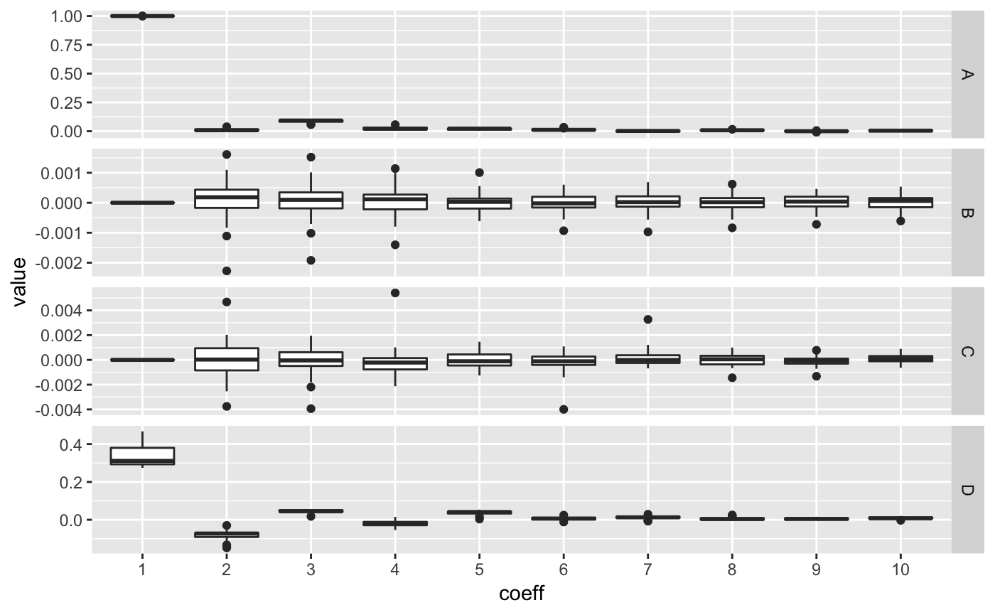
Now, we can calculate a PCA on the Coe object and plot it, along with morphospaces, calculated on the fly.

bot.p <- PCA(bot.f)
class(bot.p)        # a PCA object, let's plot it
plot(bot.p)

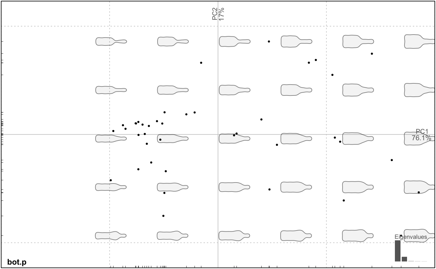
## [1] "PCA"    "prcomp"

Amazing but we will do much better afterwards.

The question of normalization in elliptical Fourier transforms is central: have a look to ?efourier.

You can also drop some harmonics with rm_harm. And methods that removes the bilateral (a)symmetry are implemented: rm_asym and rm_sym, while symmetry calculates some related indices.

Open outlines

Open outlines are curves. Methods actually implemented are:

npoly that fit natural polynomials;
opoly that fit orthogonal (also called Legendre’s) polynomials;
dfourier for the discrete cosine transform.

Note that opoly and npoly can only be used on simple curves, curves that have at most one y for any x coordinates, at least under a given orientation. dfourier can fit complex curves, curves “that back on their feets”.

Here, we will work on the fertile valves of olive stones, a (very partial) dataset provided by my colleagues Terral, Ivorra, and others.

They have two orthogonal views (a lateral and a dorsal view). See the paper cited in ?olea for more details. Let’s explore it a bit:

olea
pile(olea, ~view)    # a family picture colored by a factor

## Opn (curves)
##   - 210 curves, 99 +/- 4 coords (in $coo)
##   - 4 classifiers (in $fac): 
## # A tibble: 210 x 4
##   var   domes view  ind  
##   <fct> <fct> <fct> <fct>
## 1 Aglan cult  VD    O10  
## 2 Aglan cult  VL    O10  
## 3 Aglan cult  VD    O11  
## 4 Aglan cult  VL    O11  
## 5 Aglan cult  VD    O12  
## 6 Aglan cult  VL    O12  
## # ... with 204 more rows
##   - also: $ldk

Now, we gonna calculate opoly on it and plot the result of the PCA. Notice how consistent is the grammar and the objects obtained:

op <- opoly(olea)           # orthogonal polynomials
class(op)                   # an OpnCoe, but also a Coe
op.p <- PCA(op)             # we calculate a PCA on it
class(op.p)                 # a PCA object
op %>% PCA %>% plot(~domes+var)   # notice the formula interface to combine factors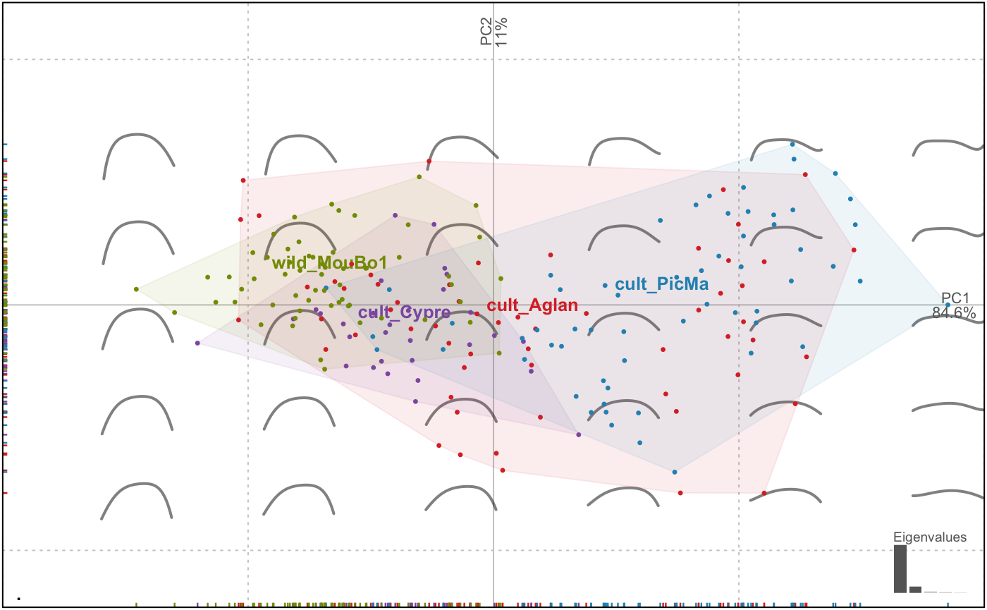

## [1] "OpnCoe" "Coe"   
## [1] "PCA"    "prcomp"

But this is perfectly wrong! We merged the two views are if they were different individuals. Momocs can first chop or filter the whole dataset to separate the two views, do morphometrics on them, and combine them afterwards.

with(olea$fac, table(view, var))
# we drop 'Cypre' since there is no VL for 'Cypre' var
olea %>% filter(var != "Cypre") %>%
# split, do morphometrics, combine
chop(~view) %>% opoly %>% combine() %T>%
# we print the OpnCoe object, then resume to the pipe
print() %>%
# note the two views in the morphospace
PCA() %>% plot_PCA(~var)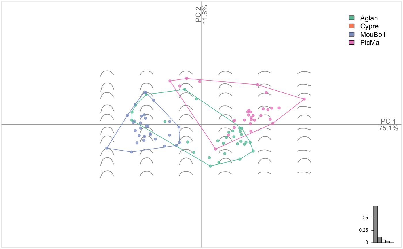

##     var
## view Aglan Cypre MouBo1 PicMa
##   VD    30    30     30    30
##   VL    30     0     30    30
## An OpnCoe object [ combined: opoly + opoly analyses ]
## --------------------
##  - $coe: 90 open outlines described
##  - $baseline1: (-0.5; 0; -0.5; 0)
##  - $baseline2: (0.5; 0; 0.5; 0)
## # A tibble: 90 x 4
##   var   domes view  ind  
##   <fct> <fct> <fct> <fct>
## 1 Aglan cult  VD    O10  
## 2 Aglan cult  VD    O11  
## 3 Aglan cult  VD    O12  
## 4 Aglan cult  VD    O13  
## 5 Aglan cult  VD    O14  
## 6 Aglan cult  VD    O15  
## # ... with 84 more rows

Now the PCA is done on the combination of two OpnCoe objects, each one resulting from an independant opoly call. That is the meaning of the [ combined: opoly + opoly analyses ] printed by the pipe above. Momocs can combine up to four different views.

Configuration of landmarks

_Landmarks methods are still quite experimental (i.e. not tested extensively)

Let’s have a look to graphics facilities and apply a full generalized Procrustes adjustment:

pile(wings)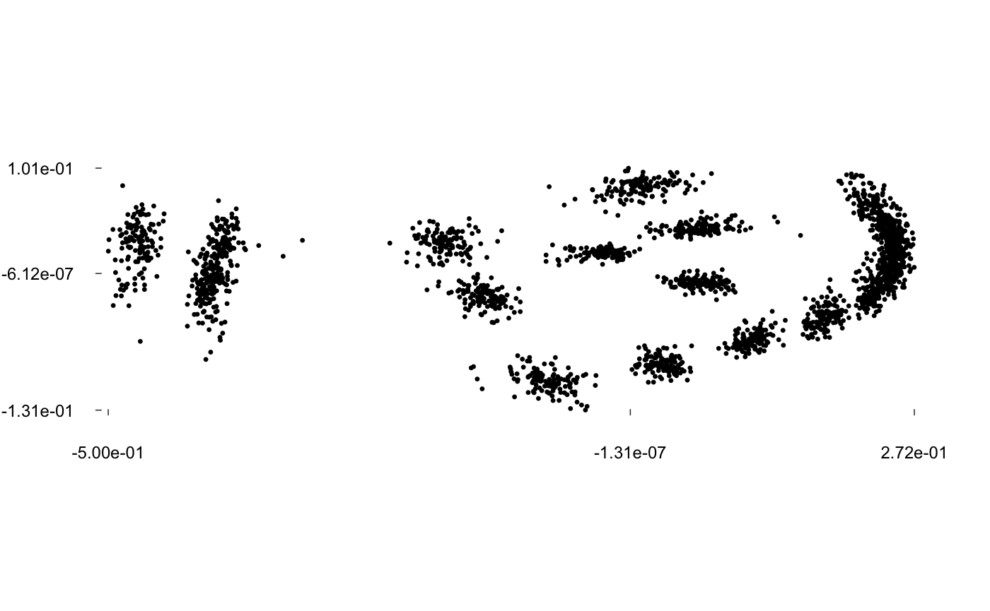

options(Momocs_verbose=FALSE) # to silent Momocs
w.al <- fgProcrustes(wings)
pile(w.al)

# PCA
PCA(w.al) %>% plot_PCA(1)

Sliding landmarks are supported and rely on geomorph package by Adams and colleagues.

pile(chaff)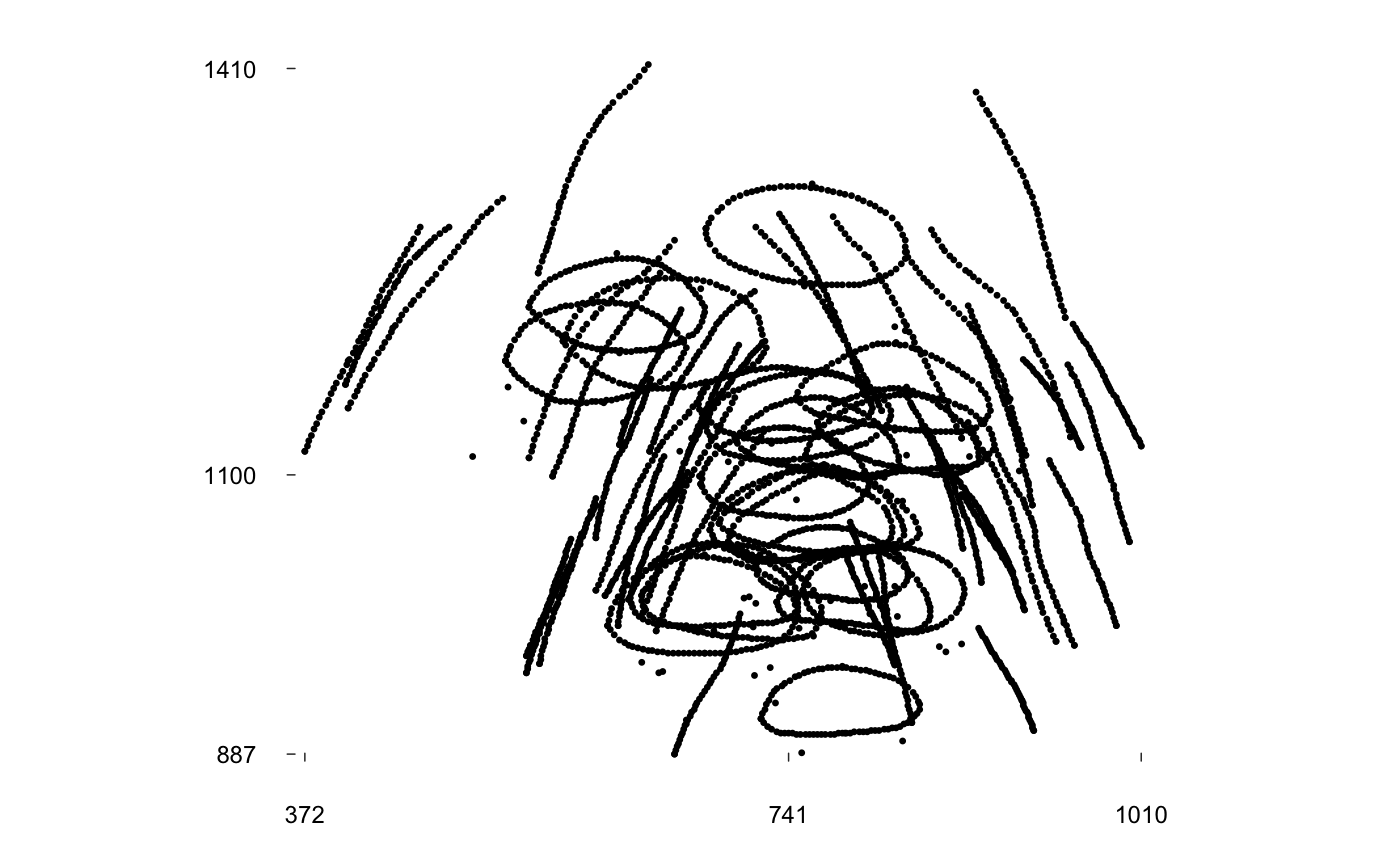

chaff.al <- fgsProcrustes(chaff)
pile(chaff.al)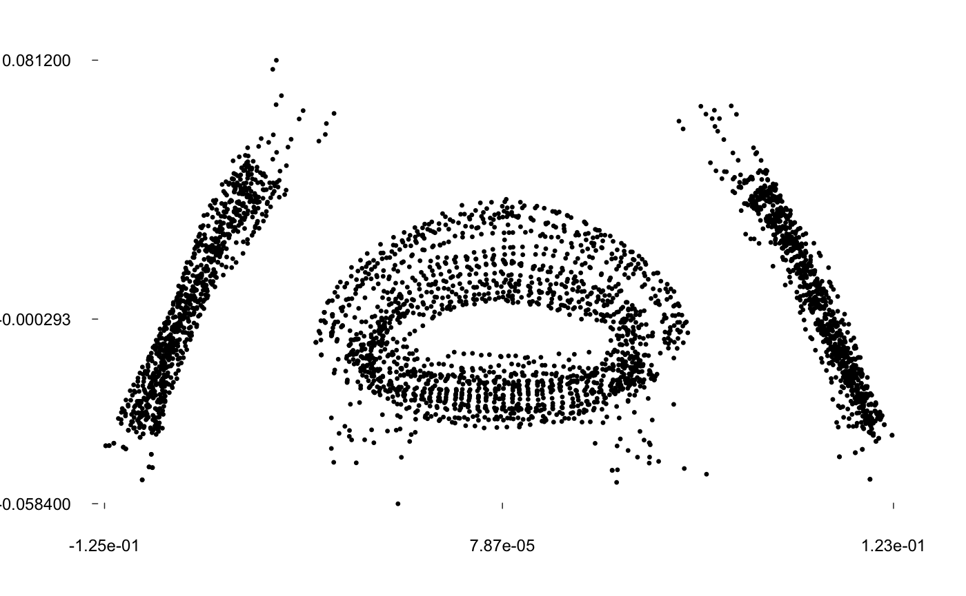

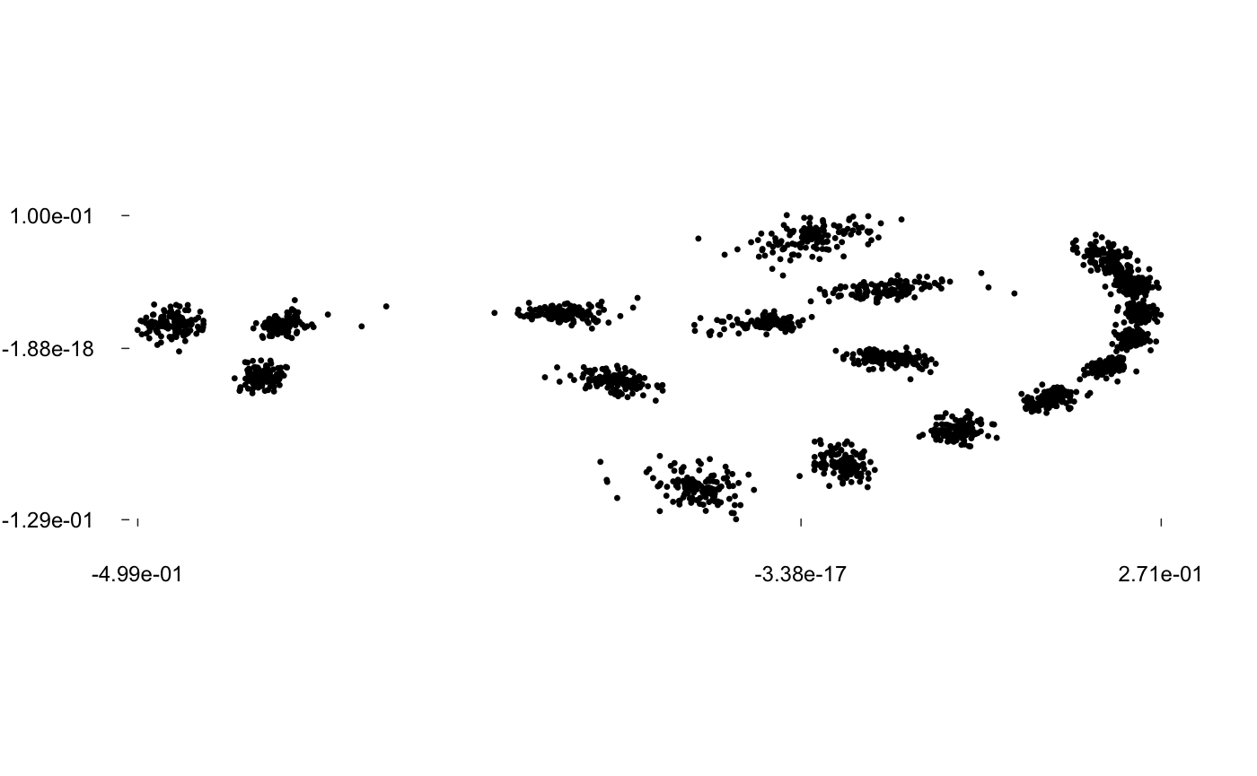
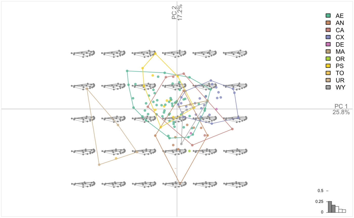
chaff.al %>% PCA() %>% plot_PCA(~taxa, chullfilled = TRUE)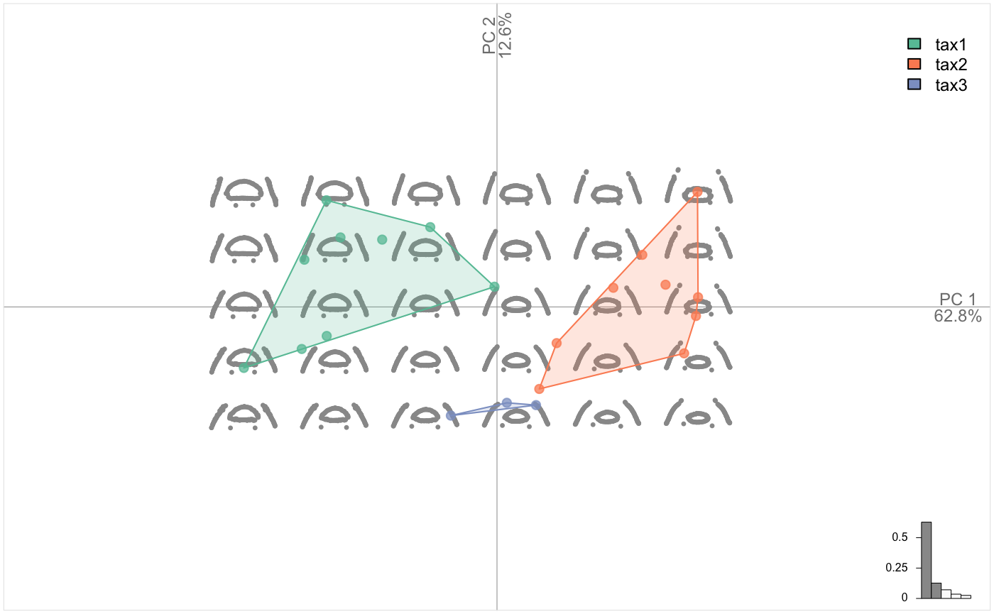

## 
  |                                                                       
  |                                                                 |   0%
  |                                                                       
  |=============                                                    |  20%
  |                                                                       
  |==========================                                       |  40%
  |                                                                       
  |=======================================                          |  60%
  |                                                                       
  |====================================================             |  80%
  |                                                                       
  |=================================================================| 100%

Again, the grammar is consistent for landmarks.

Traditional morphometrics

Traditional morphometrics lose geometries: from the variables, you can’t unambiguously reconstruct the shape. Every shape is described by a combination of measurements, (inter landmark distance, quantitative variables, scalar descriptor, etc.)

Momocs provides some basics utilities to work with such objects in the TraCoe class. There is not TraCoo per se but it can be obtained from any Coo with the measure method. Let’s take the hearts dataset that comes from handdrawn heart shapes from my former colleagues at the French Intitute of Pondicherry:

hearts
panel(hearts, fac="aut", names="aut")

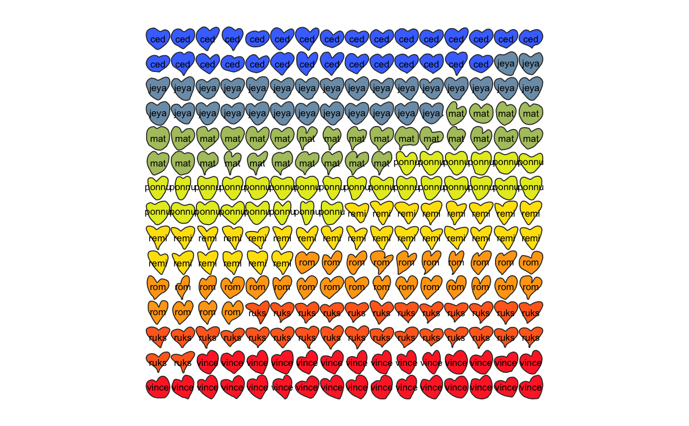
## Out (outlines)
##   - 240 outlines, 80 +/- 0 coords (in $coo)
##   - 1 classifiers (in $fac): 
## # A tibble: 240 x 1
##   aut  
##   <fct>
## 1 ced  
## 2 ced  
## 3 ced  
## 4 ced  
## 5 ced  
## 6 ced  
## # ... with 234 more rows
##   - also: $ldk

Notice that there are 4 landmarks defined on them. Such landmarks on outlines can be: defined withdef_ldk(), retrieved with get_ldk(), and overall used to align outlines with fgProcrustes(). You can compare: hearts %>% stack() with hearts %>% fgProcrustes() %>% coo_slide(ldk=1) %>% stack().

Let’s describe these hearts with scalar descriptors: area, circularity and the distance between the 1st and the 3rd bumps of the hearts. measure is of great help. Note the loadings.

ht <- measure(hearts, coo_area, coo_circularity, d(1, 3))
class(ht)
ht$coe
ht %>% PCA() %>% plot_PCA(~aut)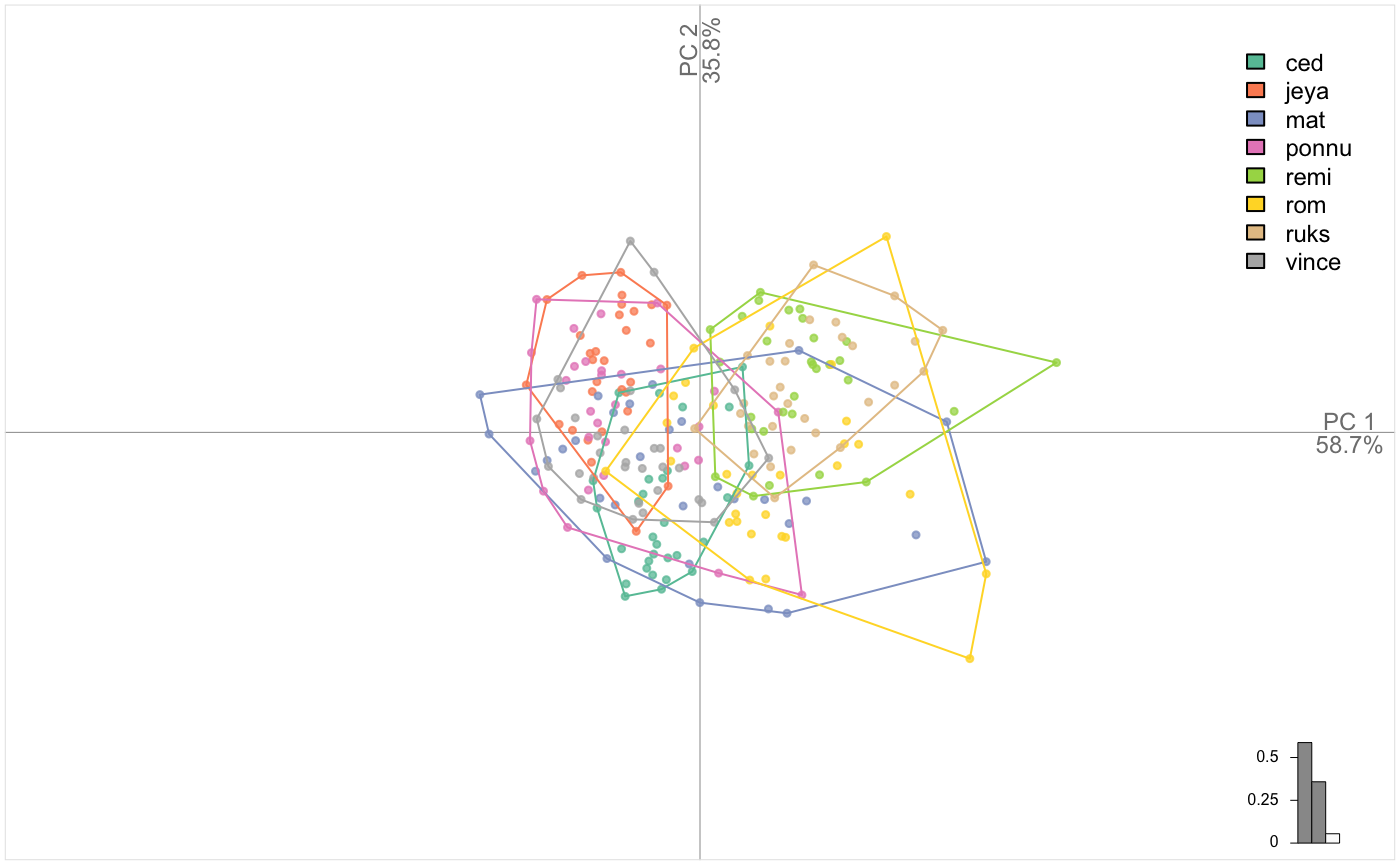

## [1] "TraCoe" "Coe"   
## # A tibble: 240 x 3
##     area circularity   d1.3
##  * <dbl>       <dbl>  <dbl>
##  1 0.627        14.0 0.0695
##  2 0.593        14.5 0.0639
##  3 0.611        16.1 0.0699
##  4 0.539        15.7 0.0627
##  5 0.541        13.6 0.0613
##  6 0.611        16.0 0.0692
##  7 0.617        16.5 0.0755
##  8 0.535        15.8 0.0655
##  9 0.521        14.3 0.0622
## 10 0.546        15.2 0.0642
## # ... with 230 more rows

Again, there are plenty of scalar descriptors of shape, which names starts with coo_*, apropos("coo_"). Have a look to the coo_vignette, see vignette("Momocs_coo").

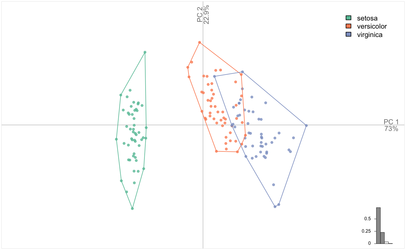
Such a TraCoe is provided in the flower dataset which is simply a rearranged iris. Once again, note the grammar consistency.

flower
flower %>% PCA() %>% plot_PCA(~sps)

You can build your own TraCoe with coo_scalars:

bot_sc <- bot %>% coo_scalars %>% TraCoe(fac=bot$fac)
bot_sc %>% PCA %>% plot_PCA(~type)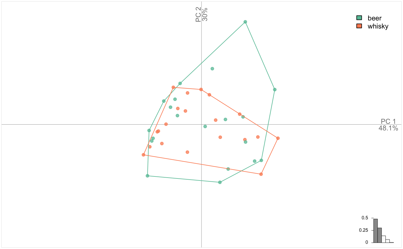

Note that, by default, PCA on TraCoe object first centers and scales variables. This can be changed, see ?PCA.

Multivariate statistics

This section will mainly be illustrated with bot, and consequently outline analysis, but it works exactly the same on any Coe object, resulting from open outlines, configuration of landmarks, traditional morphometrics, etc.

bot.f <- efourier(bot)

`PCA`: Principal Component Analysis

Let’s see the main components of shape variability with a Principal Component Analysis.

bot.p <- PCA(bot.f)
plot_PCA(bot.p)

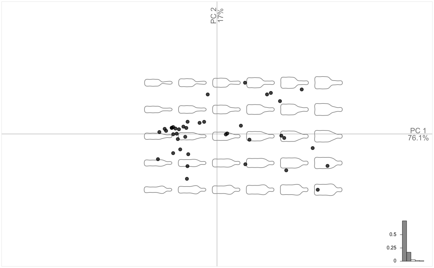
Morphological spaces are reconstructed on the fly with plot.PCA. We call it plot.PCA because it uses the familiar plot but on the particular PCA class (type class(bot.p)). We may want to display the two groups saved in bot$fac. Just type the id of the column or its name.

plot_PCA(bot.p, ~type) # there are many ways to pass the factor, see ?plot_PCA and ?fac_dispatcher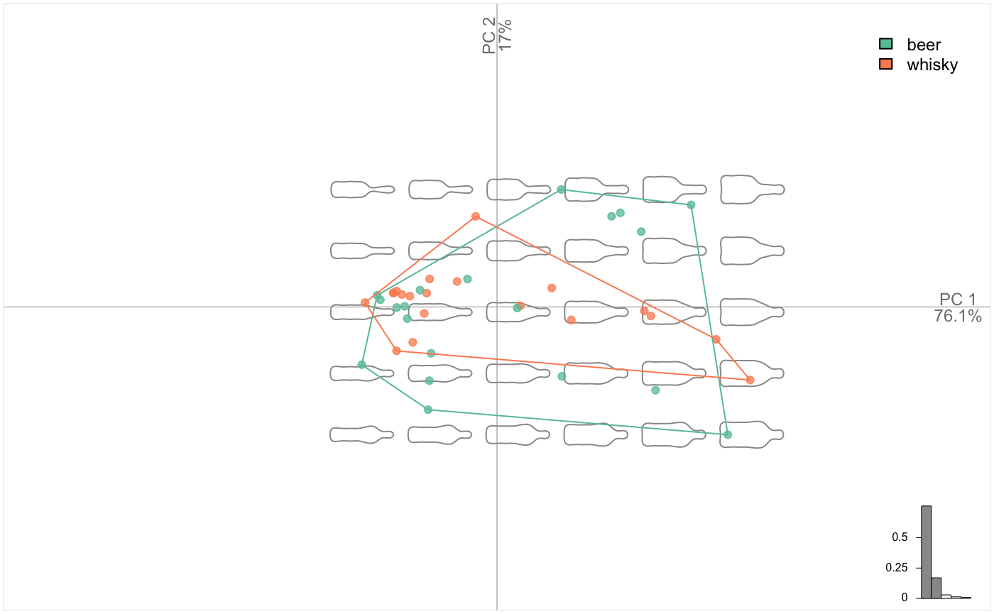

See ?plot_PCA for much more complex graphics. And also these helper functions for the PCA class:

scree(bot.p)
scree_plot(bot.p)
boxplot(bot.p, 1)
PCcontrib(bot.p)

You can also export the PCA object as a .txt file (see ?export) or as a data_frame for further use with R with:

bot.p %>% as_df(3) # The first three PCs

## # A tibble: 40 x 5
##    type   fake      PC1       PC2      PC3
##    <fct>  <fct>   <dbl>     <dbl>    <dbl>
##  1 whisky a     -0.0528 -0.0231    0.00245
##  2 whisky a     -0.0369  0.00725  -0.00866
##  3 whisky a      0.0809 -0.00479  -0.00222
##  4 whisky a     -0.0694  0.00229  -0.0158 
##  5 whisky a     -0.0112  0.0476   -0.0127 
##  6 whisky a      0.115  -0.0170   -0.0103 
##  7 whisky a     -0.0443 -0.0186   -0.00496
##  8 whisky a      0.0287  0.00996  -0.0114 
##  9 whisky a      0.0123  0.000603  0.00364
## 10 whisky a     -0.0458  0.00564  -0.00889
## # ... with 30 more rows

By the way, you can use Momocs plotters to plot non-morphometric datasets. Using a TraCoe object is an option, but PCA also works fine. Let’s see an example with iris dataset:

TraCoe(iris[, -5], fac=data.frame(sp=iris$Species)) %>%
PCA() %>% plot_PCA(~sp)

`LDA`: Linear Discriminant Analysis

We can also calculate a Linear Discriminant Analysis on the PCA scores, or on the Coe object, directly on the matrix of coefficients (and results may be better yet we may encounter collinearity between variables). Try the following:

#LDA(bot.f, 1)
# we work on PCA scores
bot.l <- LDA(bot.p, 1)
# print a summary, along with the leave-one-out cross-validation table.
bot.l
# a much more detailed summary
bot.l %>% summary
# plot.LDA works pretty much with the same grammar as plot.PCA
# here we only have one LD
plot(bot.l)
# plot the cross-validation table
plot_CV(bot.l)  # tabular version

You can also export turn it into a data_frame with as_df.

`MANOVA`: Multivariate Analysis of (co)variace

We can test for a difference in the distribution of PC scores with:

MANOVA(bot.p,  ~type)

##           Df Hotelling-Lawley approx F num Df den Df   Pr(>F)    
## fac        1           2.8388   12.977      7     32 8.88e-08 ***
## Residuals 38                                                     
## ---
## Signif. codes:  0 '***' 0.001 '**' 0.01 '*' 0.05 '.' 0.1 ' ' 1

We can also calculate pairwise combination between every levels of a fac. Here we just have two levels, so a single pairwise combination but the syntax is:

MANOVA_PW(bot.p, ~type)

## $stars.tab
##      beer whisky
## beer      ***   
## 
## $summary (see also $manovas)
##               Df Pillai approx F num Df den Df   Pr(>F)
## beer - whisky  1 0.7395    12.98      7     32 8.88e-08

If we want a MANCOVA instead :

bot %<>% mutate(cs=coo_centsize(.))
bot %>% efourier %>% PCA %>% MANOVA(~cs)

##           Df Hotelling-Lawley approx F num Df den Df Pr(>F)
## fac        1          0.32229   1.4733      7     32  0.212
## Residuals 38

`CLUST`: Hierarchical clustering

A hierarchical classification now. It relies on dist + hclust + ape::plot.phylo.

CLUST(bot.p, ~type)

Monophyly is plotted by default. Many options can be found in ?CLUST

`KMEANS`: K-means clustering

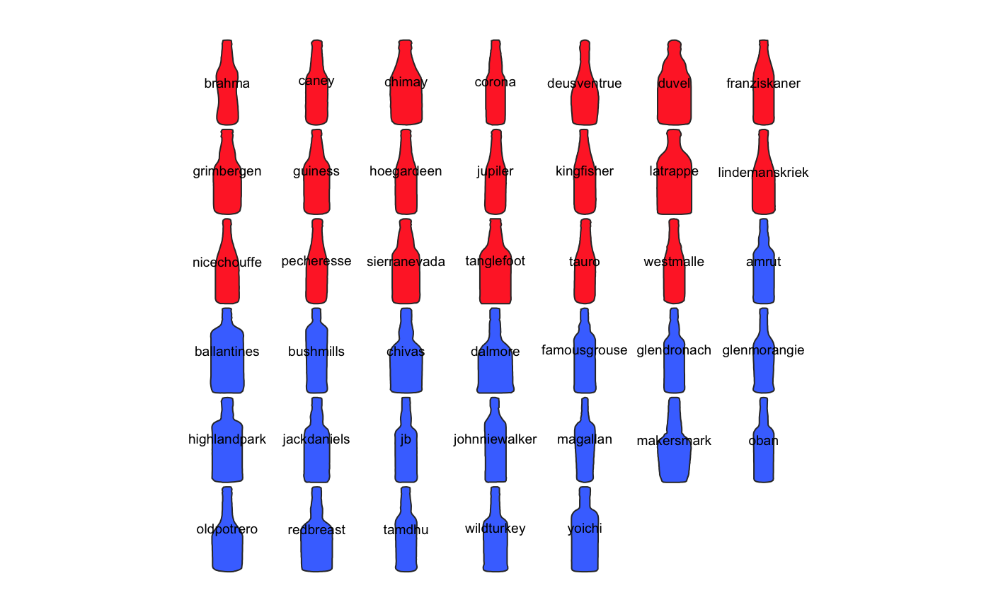
A very minimal k-means clustering is implemented:

KMEANS(bot.p, centers = 5)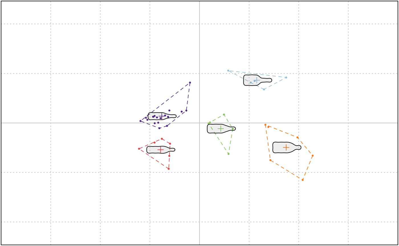

## K-means clustering with 5 clusters of sizes 5, 5, 6, 6, 18
## 
## Cluster means:
##           PC1          PC2
## 1  0.06730453  0.050371247
## 2  0.02497106 -0.006671549
## 3 -0.04573875 -0.031541607
## 4  0.10184224 -0.028875902
## 5 -0.04433327  0.008000365
## 
## Clustering vector:
##         brahma          caney         chimay         corona    deusventrue 
##              3              5              4              5              5 
##          duvel   franziskaner     grimbergen        guiness     hoegardeen 
##              4              3              2              2              5 
##        jupiler     kingfisher       latrappe lindemanskriek    nicechouffe 
##              5              5              4              5              5 
##     pecheresse   sierranevada     tanglefoot          tauro      westmalle 
##              5              2              4              5              5 
##          amrut    ballantines      bushmills         chivas        dalmore 
##              5              4              3              1              1 
##   famousgrouse    glendronach   glenmorangie   highlandpark    jackdaniels 
##              3              5              5              4              2 
##             jb  johnniewalker       magallan     makersmark           oban 
##              5              3              3              1              5 
##     oldpotrero      redbreast         tamdhu     wildturkey         yoichi 
##              1              1              5              5              2 
## 
## Within cluster sum of squares by cluster:
## [1] 0.002720829 0.001916822 0.001860776 0.006121728 0.006537571
##  (between_SS / total_SS =  89.4 %)
## 
## Available components:
## 
## [1] "cluster"      "centers"      "totss"        "withinss"    
## [5] "tot.withinss" "betweenss"    "size"         "iter"        
## [9] "ifault"

`MSHAPES`: Mean shapes

We can retrieve the mean shapes, group wise (if a fac is specified), or the global mean shape (if omitted). It works from the Coe object:

# mean shape
bot.f %>% MSHAPES() %>% coo_plot()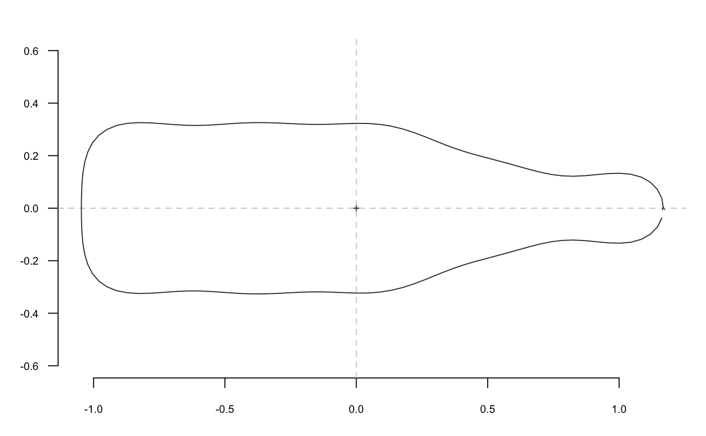

# mean shape, per group
bot.ms <- MSHAPES(bot.f, ~type)
# lets rebuild an Out
Out(bot.ms$shp) %>% panel(names=TRUE)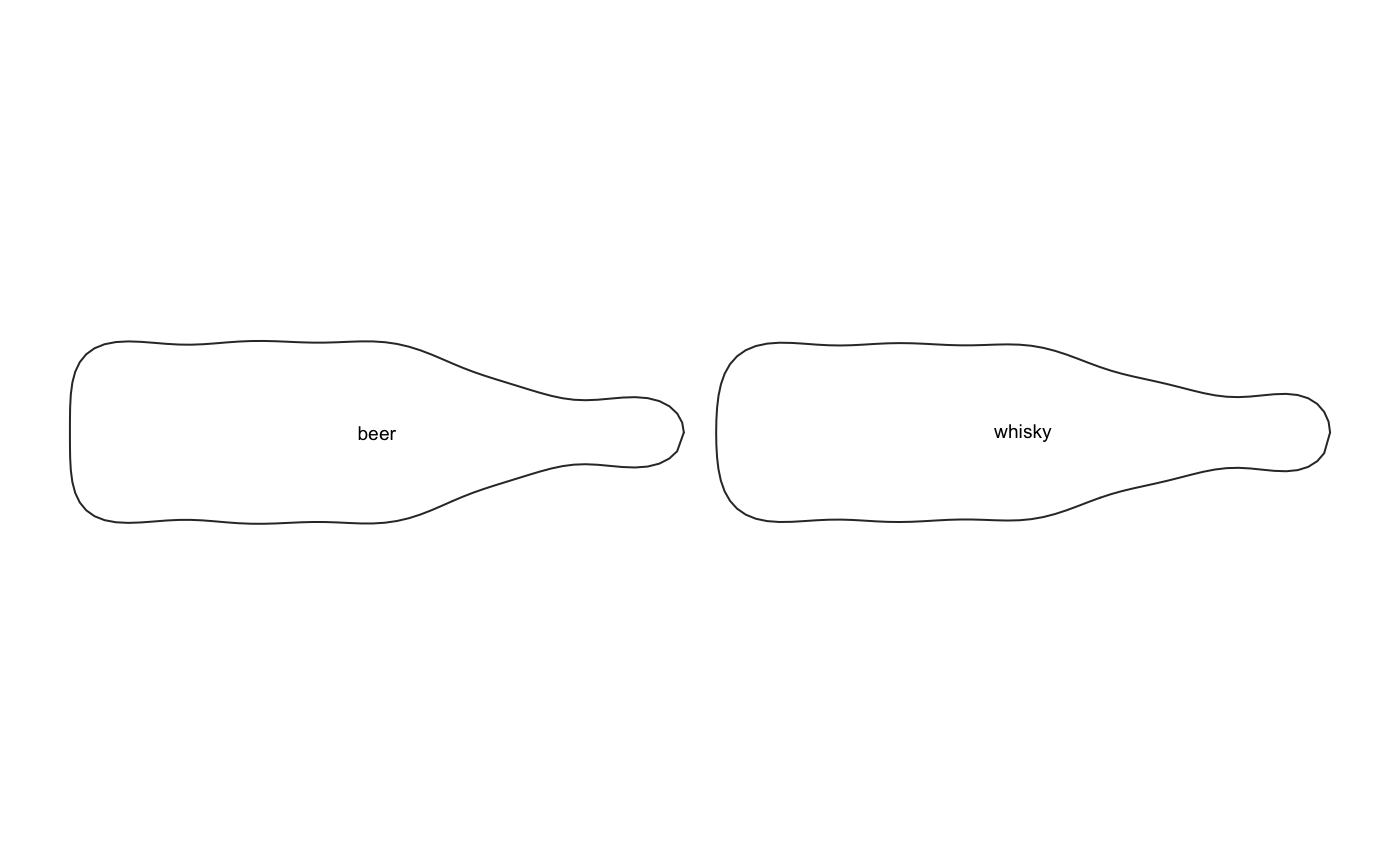

# or individual shapes
beer   <- bot.ms$shp$beer    %>% coo_plot(border="blue")
whisky <- bot.ms$shp$whisky  %>% coo_draw(border="red")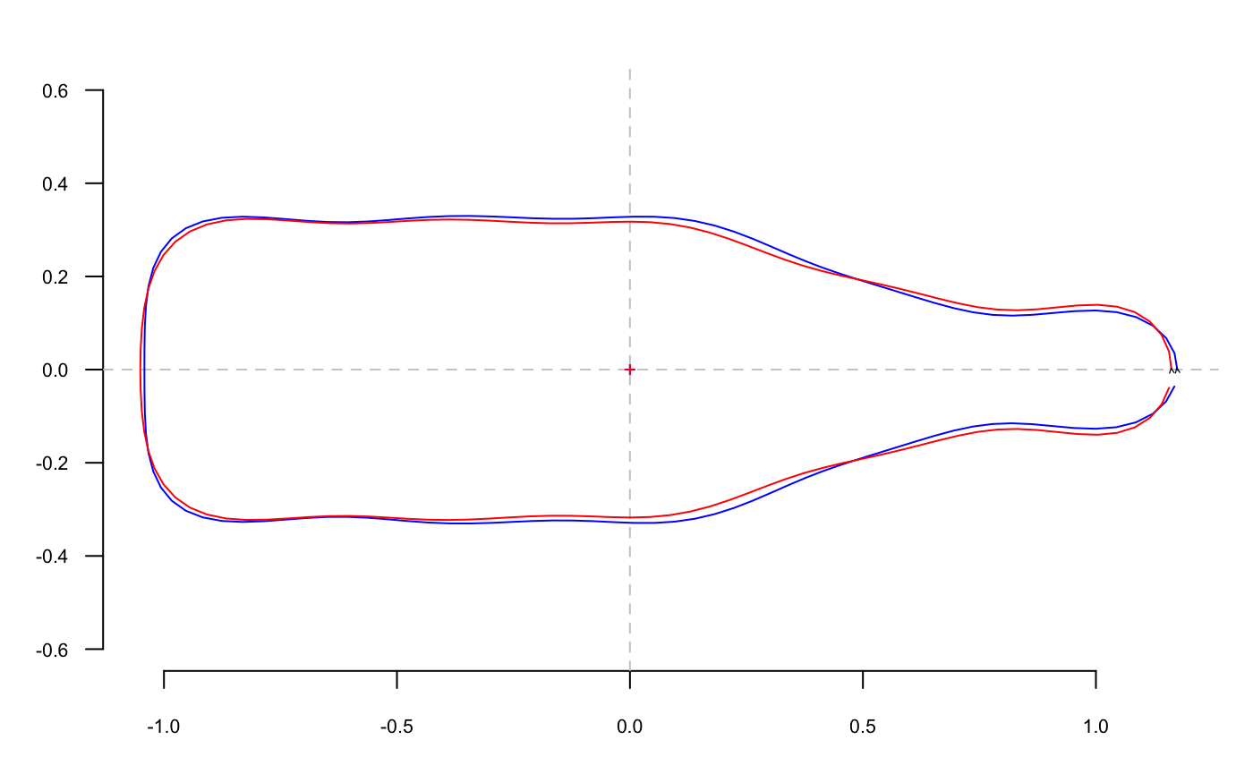

We can also plot a pairwise comparison of them:

leaves <- shapes %>% slice(grep("leaf", names(shapes))) %$% coo
leaves %>% plot_MSHAPES()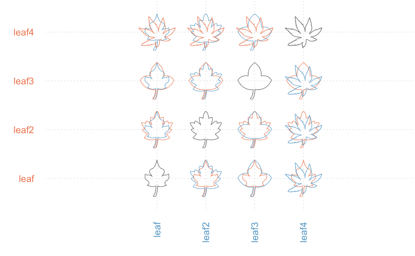

# or from mshapes directly
bot %>% efourier(6) %>% MSHAPES(~type) %>% plot_MSHAPES()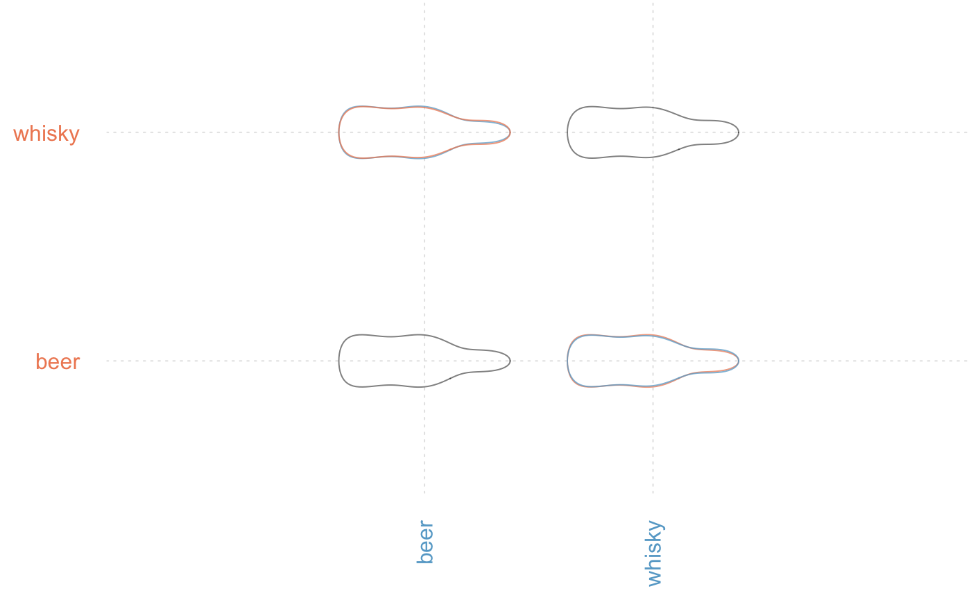

Manipulating objects

One common yet boring task of morphometrics consists in handling datasets: add new information, remove some individuals, etc.

Momocs adapts dplyr verbs to its objects, and add new ones. If you have never heard of dplyr, let’s have a look to its introduction there, this may change your (R) life.

data(olea)
olea

## Opn (curves)
##   - 210 curves, 99 +/- 4 coords (in $coo)
##   - 4 classifiers (in $fac): 
## # A tibble: 210 x 4
##   var   domes view  ind  
##   <fct> <fct> <fct> <fct>
## 1 Aglan cult  VD    O10  
## 2 Aglan cult  VL    O10  
## 3 Aglan cult  VD    O11  
## 4 Aglan cult  VL    O11  
## 5 Aglan cult  VD    O12  
## 6 Aglan cult  VL    O12  
## # ... with 204 more rows
##   - also: $ldk

`mutate`: add new columns

mutate(olea, fake=factor(rep(letters[1:2], each=105)))

## Opn (curves)
##   - 210 curves, 99 +/- 4 coords (in $coo)
##   - 5 classifiers (in $fac): 
## # A tibble: 210 x 5
##   var   domes view  ind   fake 
##   <fct> <fct> <fct> <fct> <fct>
## 1 Aglan cult  VD    O10   a    
## 2 Aglan cult  VL    O10   a    
## 3 Aglan cult  VD    O11   a    
## 4 Aglan cult  VL    O11   a    
## 5 Aglan cult  VD    O12   a    
## 6 Aglan cult  VL    O12   a    
## # ... with 204 more rows
##   - also: $ldk

`slice`: select individuals based on their position

slice(olea, 1:5)

## Opn (curves)
##   - 5 curves, 99 +/- 4 coords (in $coo)
##   - 4 classifiers (in $fac): 
## # A tibble: 5 x 4
##   var   domes view  ind  
##   <fct> <fct> <fct> <fct>
## 1 Aglan cult  VD    O10  
## 2 Aglan cult  VL    O10  
## 3 Aglan cult  VD    O11  
## 4 Aglan cult  VL    O11  
## 5 Aglan cult  VD    O12  
##   - also: $ldk

slice(olea, -(1:100))

## Opn (curves)
##   - 110 curves, 99 +/- 4 coords (in $coo)
##   - 4 classifiers (in $fac): 
## # A tibble: 110 x 4
##   var   domes view  ind  
##   <fct> <fct> <fct> <fct>
## 1 PicMa cult  VD    O15  
## 2 PicMa cult  VL    O15  
## 3 PicMa cult  VD    O16  
## 4 PicMa cult  VL    O16  
## 5 PicMa cult  VD    O17  
## 6 PicMa cult  VL    O17  
## # ... with 104 more rows
##   - also: $ldk

`filter`: select individual based on a logical condition

filter(olea, domes=="cult")

## Opn (curves)
##   - 150 curves, 99 +/- 3 coords (in $coo)
##   - 4 classifiers (in $fac): 
## # A tibble: 150 x 4
##   var   domes view  ind  
##   <fct> <fct> <fct> <fct>
## 1 Aglan cult  VD    O10  
## 2 Aglan cult  VL    O10  
## 3 Aglan cult  VD    O11  
## 4 Aglan cult  VL    O11  
## 5 Aglan cult  VD    O12  
## 6 Aglan cult  VL    O12  
## # ... with 144 more rows
##   - also: $ldk

# %in% is useful
filter(olea, var %in% c("Aglan", "Cypre"))

## Opn (curves)
##   - 90 curves, 99 +/- 4 coords (in $coo)
##   - 4 classifiers (in $fac): 
## # A tibble: 90 x 4
##   var   domes view  ind  
##   <fct> <fct> <fct> <fct>
## 1 Aglan cult  VD    O10  
## 2 Aglan cult  VL    O10  
## 3 Aglan cult  VD    O11  
## 4 Aglan cult  VL    O11  
## 5 Aglan cult  VD    O12  
## 6 Aglan cult  VL    O12  
## # ... with 84 more rows
##   - also: $ldk

# or its complement
filter(olea, !(var %in% c("Aglan", "Cypre")))

## Opn (curves)
##   - 120 curves, 99 +/- 3 coords (in $coo)
##   - 4 classifiers (in $fac): 
## # A tibble: 120 x 4
##   var   domes view  ind  
##   <fct> <fct> <fct> <fct>
## 1 PicMa cult  VD    O10  
## 2 PicMa cult  VL    O10  
## 3 PicMa cult  VD    O11  
## 4 PicMa cult  VL    O11  
## 5 PicMa cult  VD    O12  
## 6 PicMa cult  VL    O12  
## # ... with 114 more rows
##   - also: $ldk

# Also works with more than one condition
filter(olea, domes=="cult", view!="VD")

## Opn (curves)
##   - 60 curves, 97 +/- 4 coords (in $coo)
##   - 4 classifiers (in $fac): 
## # A tibble: 60 x 4
##   var   domes view  ind  
##   <fct> <fct> <fct> <fct>
## 1 Aglan cult  VL    O10  
## 2 Aglan cult  VL    O11  
## 3 Aglan cult  VL    O12  
## 4 Aglan cult  VL    O13  
## 5 Aglan cult  VL    O14  
## 6 Aglan cult  VL    O15  
## # ... with 54 more rows
##   - also: $ldk

# or on operation on numeric, here a dummy numeric column
olea %>% mutate(foo=1:210) %>% filter(foo<12)

## Opn (curves)
##   - 11 curves, 99 +/- 5 coords (in $coo)
##   - 5 classifiers (in $fac): 
## # A tibble: 11 x 5
##   var   domes view  ind     foo
##   <fct> <fct> <fct> <fct> <int>
## 1 Aglan cult  VD    O10       1
## 2 Aglan cult  VL    O10       2
## 3 Aglan cult  VD    O11       3
## 4 Aglan cult  VL    O11       4
## 5 Aglan cult  VD    O12       5
## 6 Aglan cult  VL    O12       6
## # ... with 5 more rows
##   - also: $ldk

olea %>% mutate(foo=1:210) %>% filter(foo>median(foo))

## Opn (curves)
##   - 105 curves, 99 +/- 4 coords (in $coo)
##   - 5 classifiers (in $fac): 
## # A tibble: 105 x 5
##   var   domes view  ind     foo
##   <fct> <fct> <fct> <fct> <int>
## 1 PicMa cult  VL    O17     106
## 2 PicMa cult  VD    O18     107
## 3 PicMa cult  VL    O18     108
## 4 PicMa cult  VD    O19     109
## 5 PicMa cult  VL    O19     110
## 6 PicMa cult  VD    O1      111
## # ... with 99 more rows
##   - also: $ldk

`select`: pick, reorder columns from the $fac

# reorder columns
select(olea, view, domes, var, ind)
# drop some and show the use of numeric index
select(olea, 1, Ind=ind)
# drop one
select(olea, -ind)

## Opn (curves)
##   - 210 curves, 99 +/- 4 coords (in $coo)
##   - 4 classifiers (in $fac): 
## # A tibble: 210 x 4
##   view  domes var   ind  
##   <fct> <fct> <fct> <fct>
## 1 VD    cult  Aglan O10  
## 2 VL    cult  Aglan O10  
## 3 VD    cult  Aglan O11  
## 4 VL    cult  Aglan O11  
## 5 VD    cult  Aglan O12  
## 6 VL    cult  Aglan O12  
## # ... with 204 more rows
##   - also: $ldk
## Opn (curves)
##   - 210 curves, 99 +/- 4 coords (in $coo)
##   - 2 classifiers (in $fac): 
## # A tibble: 210 x 2
##   var   Ind  
##   <fct> <fct>
## 1 Aglan O10  
## 2 Aglan O10  
## 3 Aglan O11  
## 4 Aglan O11  
## 5 Aglan O12  
## 6 Aglan O12  
## # ... with 204 more rows
##   - also: $ldk
## Opn (curves)
##   - 210 curves, 99 +/- 4 coords (in $coo)
##   - 3 classifiers (in $fac): 
## # A tibble: 210 x 3
##   var   domes view 
##   <fct> <fct> <fct>
## 1 Aglan cult  VD   
## 2 Aglan cult  VL   
## 3 Aglan cult  VD   
## 4 Aglan cult  VL   
## 5 Aglan cult  VD   
## 6 Aglan cult  VL   
## # ... with 204 more rows
##   - also: $ldk

And you can pipe those operations: say, we only want dorsal views from domesticated individuals, for a (renamed) ‘status’ column, and drop the ‘ind’ column:

olea %>%
filter(domes=="cult", view=="VD") %>%
rename(domesticated=domes) %>%
select(-ind)

## Opn (curves)
##   - 90 curves, 100 +/- 2 coords (in $coo)
##   - 3 classifiers (in $fac): 
## # A tibble: 90 x 3
##   var   domesticated view 
##   <fct> <fct>        <fct>
## 1 Aglan cult         VD   
## 2 Aglan cult         VD   
## 3 Aglan cult         VD   
## 4 Aglan cult         VD   
## 5 Aglan cult         VD   
## 6 Aglan cult         VD   
## # ... with 84 more rows
##   - also: $ldk

You can also use dplyr verbs on the fac directly, eg:

olea$fac %>% dplyr::group_by(var) %>% 
  dplyr::mutate(n=1:n(), N=n())

## # A tibble: 210 x 6
## # Groups:   var [4]
##    var   domes view  ind       n     N
##    <fct> <fct> <fct> <fct> <int> <int>
##  1 Aglan cult  VD    O10       1    60
##  2 Aglan cult  VL    O10       2    60
##  3 Aglan cult  VD    O11       3    60
##  4 Aglan cult  VL    O11       4    60
##  5 Aglan cult  VD    O12       5    60
##  6 Aglan cult  VL    O12       6    60
##  7 Aglan cult  VD    O13       7    60
##  8 Aglan cult  VL    O13       8    60
##  9 Aglan cult  VD    O14       9    60
## 10 Aglan cult  VL    O14      10    60
## # ... with 200 more rows

If you want to save it, do not forget to reassign it back to the $fac: olea$fac <- olea$fac %>% some_operations or even olea$fac %<>% some_operations.

Note that if you due to namespace conflicts, if you use dplyr, and in a larger extent the tidyverse you must use library(dplyr) (or library(tydyverse)) before library(Momocs).

That being said, the adaptation of these dplyr verbs should save time and some headaches.

New verbs are implemented: for instance, you can chop (a split on Coo objects) according to a condition: this will create a list, on which you can apply further operations, then combine it back. This is particularly useful when you want to apply independant treatments to different partitions, eg orthogonal views of your model. Prior to this, we can use table to cross-tabulate data from $fac. We could have done the first step of what follows with rm_uncomplete that drops (if any) missing data.

with(olea$fac, table(var, view))
# we drop 'Cypre' since there is no VL for 'Cypre' var
olea %>% 
  filter(var != "Cypre") %>%
  # split, do morphometrics, combine
  chop(~view) %>% opoly %>% combine() %>%
  # note the two views in the morphospace
  PCA() %>% plot_PCA(~var)

##         view
## var      VD VL
##   Aglan  30 30
##   Cypre  30  0
##   MouBo1 30 30
##   PicMa  30 30

Various helpers

Some methods help, on Coe objects to: * select groups with at least a certain number of individuals in them: at_least * removes outliers : which_out * sample a given number: sample_n; * sample a given proportion: sample_frac; * generate new individuals based on calibrated Gaussian coefficient generation: breed; * generate new individuals based on permutations: perm.

Several shortcuts are implemented on Coo and Coe objects: * names returns shape names; * length returns their number; * Ntable does the same job and plots a confusion matrix; * [] extracts one (or more) shape; * $ can access either a shape name or a column name for the $fac.

Try the following:

names(bot)
length(bot)
bot[1]
bot[1:5]
bot$brahma
bot$type

Babel import/export

There are various morphometrics formats in the wild, almost as much as softwares. Momocs tries to create bridges between them, all gathered in the Babel family.

Note that these will move to Momit/Momecs asap.

Bridges within R

You can convert from/to array, matrix, list or data.frame with the functions {a, m, l, d}2{a, m, l, d}. For instance, l2a converts a list into an array that you can use with geomorph; a2l does the inverse operation.

Imagine you want to import pupfish from geomorph as a Ldk object:

library(geomorph)
data(pupfish)
str(pupfish)
# so $coords will become $coo, and
# all other components will be turned into a data.frame to feed $fac
# with a single line
Ldk(coo=pupfish$coords %>% a2l,
  fac=pupfish[-1] %>% as.data.frame())

Import from StereoMorph

If you use StereoMorph to digitize landmarks and curves, you can import them, from the files produced with the functions import_StereoMorph_ldk and import_StereoMorph_curve.

Import from tps and other digitizing softwares

.tps files can be read with import_tps
.nts files an be read with nts2Coo (will be turned into import_nts soon)

Direct build of *Coe objects

You’re not bound with Momocs from the “shapes” step, ie you do not have to start from Coo objects. For instance if you have a matrix of coefficients, you can directly build an OutCoe with the builder (see below). Same approach for OpnCoe and TraCoe; have a look to the help files of these builders.

# we simulate an imported matrix of coordinates, eg from a .csv
coeffs_from_the_wild <- bot %>% efourier(6) %$% coe
coeffs_in_Momocs <- OutCoe(coe=coeffs_from_the_wild, method="efourier", norm=TRUE)
coeffs_in_Momocs %>% PCA %>% plot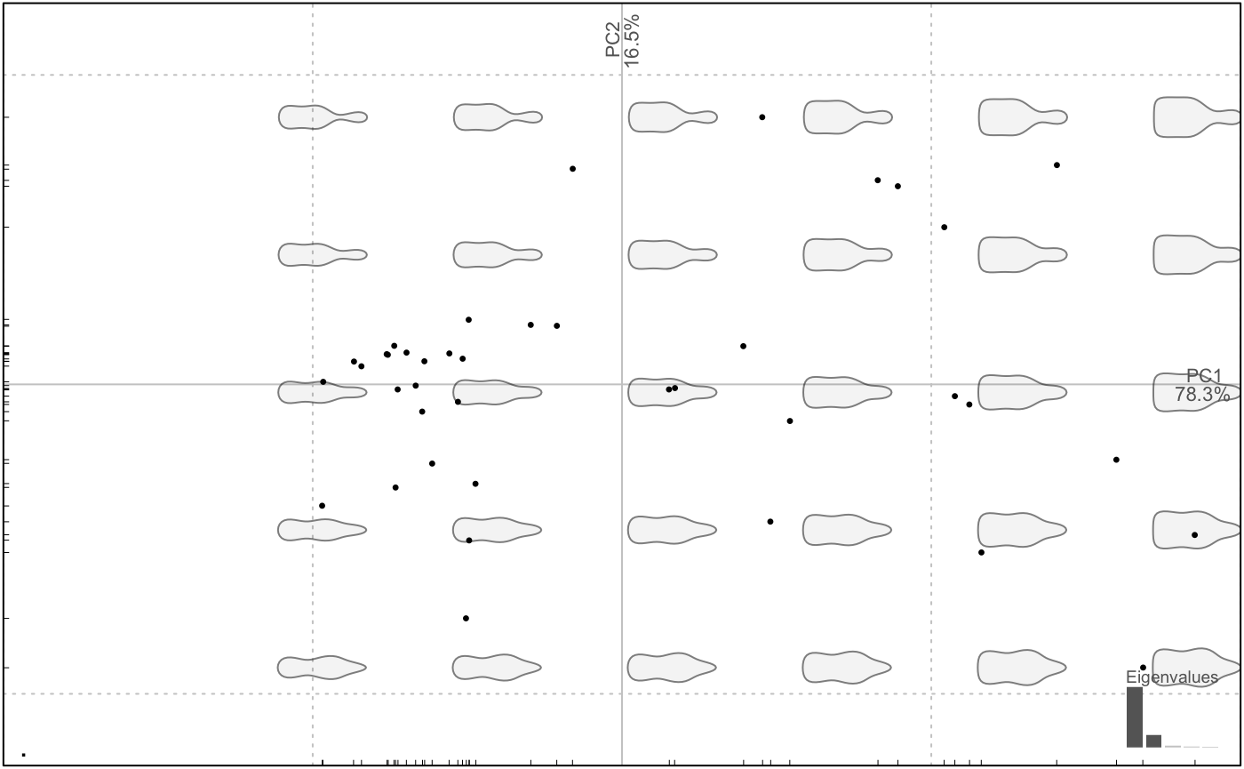

Import misc

If covariables are encoded in filenames, which is a good practice, eg if you have files named spA_group7_ind4_VL.{txt|jpg|etc.}, use lf_structure;
If you need rewriting rules on your $fac, rw_rule is your friend;
If you need to rescale imported coordinates, see rescale;
If you need to tie images (eg outlines) and .txt (eg coordinates of landmarks on them), see tie_jpg_txt.

Save from R

The best way to save a Momocs object is probably to use the base save function. You can call it back afterwards with load:

save(bot, file="Bottles.rda")
# closing R, going to the beach, back at work
load("Bottles.rda") # bot is back

Export from R

Any Momocs object, Coos, Coes, PCAs, etc. can be turned into a data.frame with as_df.

bot %>% as_df
bot %>% efourier %>% as_df
bot %>% efourier %>% PCA %>% as_df

## # A tibble: 40 x 4
##    coo             type   fake     cs
##    <list>          <fct>  <fct> <dbl>
##  1 <dbl [138 × 2]> whisky a      335.
##  2 <dbl [168 × 2]> whisky a      307.
##  3 <dbl [189 × 2]> whisky a      220.
##  4 <dbl [129 × 2]> whisky a      245.
##  5 <dbl [152 × 2]> whisky a      277.
##  6 <dbl [161 × 2]> whisky a      210.
##  7 <dbl [124 × 2]> whisky a      267.
##  8 <dbl [126 × 2]> whisky a      251.
##  9 <dbl [183 × 2]> whisky a      240.
## 10 <dbl [193 × 2]> whisky a      325.
## # ... with 30 more rows
## # A tibble: 40 x 43
##    type   fake     cs    A1      A2     A3     A4      A5      A6       A7
##    <fct>  <fct> <dbl> <dbl>   <dbl>  <dbl>  <dbl>   <dbl>   <dbl>    <dbl>
##  1 whisky a      335. 1.000 0.00677 0.0935 0.0137 0.0238  0.00859  0.00318
##  2 whisky a      307. 1.000 0.00737 0.0954 0.0145 0.0222  0.00667  0.00355
##  3 whisky a      220. 1.    0.0165  0.0757 0.0274 0.00988 0.0143  -0.00474
##  4 whisky a      245. 1.    0.00749 0.0962 0.0122 0.0229  0.00728  0.00550
##  5 whisky a      277. 1     0.0196  0.0928 0.0223 0.0153  0.0149   0.00252
##  6 whisky a      210. 1.000 0.0222  0.0690 0.0335 0.00932 0.0211  -0.00169
##  7 whisky a      267. 1.    0.00731 0.0911 0.0129 0.0231  0.0106   0.00458
##  8 whisky a      251. 1     0.00952 0.0857 0.0197 0.0129  0.00849 -0.00220
##  9 whisky a      240. 1     0.00959 0.0883 0.0227 0.0178  0.0107  -0.00152
## 10 whisky a      325. 1.000 0.00960 0.0919 0.0139 0.0201  0.00895  0.00240
## # ... with 30 more rows, and 33 more variables: A8 <dbl>, A9 <dbl>,
## #   A10 <dbl>, B1 <dbl>, B2 <dbl>, B3 <dbl>, B4 <dbl>, B5 <dbl>, B6 <dbl>,
## #   B7 <dbl>, B8 <dbl>, B9 <dbl>, B10 <dbl>, C1 <dbl>, C2 <dbl>, C3 <dbl>,
## #   C4 <dbl>, C5 <dbl>, C6 <dbl>, C7 <dbl>, C8 <dbl>, C9 <dbl>, C10 <dbl>,
## #   D1 <dbl>, D2 <dbl>, D3 <dbl>, D4 <dbl>, D5 <dbl>, D6 <dbl>, D7 <dbl>,
## #   D8 <dbl>, D9 <dbl>, D10 <dbl>
## # A tibble: 40 x 43
##    type   fake     cs     PC1      PC2      PC3      PC4      PC5      PC6
##    <fct>  <fct> <dbl>   <dbl>    <dbl>    <dbl>    <dbl>    <dbl>    <dbl>
##  1 whisky a      335. -0.0528 -2.31e-2  0.00245 -1.54e-2  6.05e-3 -9.73e-4
##  2 whisky a      307. -0.0369  7.25e-3 -0.00866 -9.21e-3 -2.77e-3 -2.82e-3
##  3 whisky a      220.  0.0809 -4.79e-3 -0.00222 -1.07e-2 -9.96e-4 -6.91e-3
##  4 whisky a      245. -0.0694  2.29e-3 -0.0158  -6.19e-3 -3.09e-4  3.86e-3
##  5 whisky a      277. -0.0112  4.76e-2 -0.0127   1.75e-2  1.35e-2 -6.99e-3
##  6 whisky a      210.  0.115  -1.70e-2 -0.0103  -9.12e-3  3.77e-4  1.26e-3
##  7 whisky a      267. -0.0443 -1.86e-2 -0.00496 -2.23e-4  1.90e-3  3.22e-3
##  8 whisky a      251.  0.0287  9.96e-3 -0.0114  -8.72e-3 -4.46e-3 -4.23e-3
##  9 whisky a      240.  0.0123  6.03e-4  0.00364 -8.19e-3 -3.91e-3  3.76e-4
## 10 whisky a      325. -0.0458  5.64e-3 -0.00889 -5.25e-3  3.99e-3 -2.42e-3
## # ... with 30 more rows, and 34 more variables: PC7 <dbl>, PC8 <dbl>,
## #   PC9 <dbl>, PC10 <dbl>, PC11 <dbl>, PC12 <dbl>, PC13 <dbl>, PC14 <dbl>,
## #   PC15 <dbl>, PC16 <dbl>, PC17 <dbl>, PC18 <dbl>, PC19 <dbl>,
## #   PC20 <dbl>, PC21 <dbl>, PC22 <dbl>, PC23 <dbl>, PC24 <dbl>,
## #   PC25 <dbl>, PC26 <dbl>, PC27 <dbl>, PC28 <dbl>, PC29 <dbl>,
## #   PC30 <dbl>, PC31 <dbl>, PC32 <dbl>, PC33 <dbl>, PC34 <dbl>,
## #   PC35 <dbl>, PC36 <dbl>, PC37 <dbl>, PC38 <dbl>, PC39 <dbl>, PC40 <dbl>

If the heretic you want to exit R to do stats elsewhere, export is your friend:

bot %>% efourier %>% export
bot %>% efourier %>% PCA %>% export

But, of course, you can directly access information within the Momocs objects; try the following:

# from Coo objects
bot$coo # list of matrices (of xy coordinates)
bot$fac # data.frame for covariates

# from Coe objects
bot.f$coe # matrix of coefficients
bot.f$fac # data.frame for covariates

# from PCA objects
bot.p$x        # scores
bot.p$rotation # rotation matrix

Graphics

Most graphics are currently being rewritten, either to pure ggplot2 or using grindr. See the dedicated embryo of vignette: see vignette("Momocs_grindr").

`tps_*`: Thin Plate Splines

TPS have not been presented before but here there are:

tps_grid(beer, whisky)
tps_arr(beer, whisky)
tps_iso(beer, whisky)

Again, plenty options in ?tps_*.

You may also like lolliplots and friends:

coo_lolli(beer, whisky); title("coo_lolli")
coo_arrows(beer, whisky); title("coo_arrow")

# an example with coo_ruban
coo_plot(beer) # to get the first plot
coo_ruban(beer, edm(beer, whisky), lwd=8) # we add ruban based from deviations
coo_draw(whisky)
title("coo_ruban")

Color palettes

Nice palettes are bundled with Momocs, see ?palettes.

Frequently asked questions

See vignette("Momocs_FAQ").

Done with love by Vincent Bonhomme <bonhomme.vincent@gmail.com>.
Help/suggestions/review/critics are welcome.
Sources are there

Vincent Bonhomme

2018-10-28