PCA plot using grindr layers

Quickly vizualise PCA objects and friends and build customs plots using the layers. See examples.

Usage

plot_PCA(
  x,
  f = NULL,
  axes = c(1, 2),
  palette = NULL,
  points = TRUE,
  points_transp = 1/4,
  morphospace = TRUE,
  morphospace_position = "range",
  chull = TRUE,
  chullfilled = FALSE,
  labelpoints = FALSE,
  labelgroups = FALSE,
  legend = TRUE,
  title = "",
  center_origin = TRUE,
  zoom = 0.9,
  eigen = TRUE,
  box = TRUE,
  axesnames = TRUE,
  axesvar = TRUE
)

Arguments

x

a PCA object

f

factor specification to feed fac_dispatcher

axes

numeric of length two to select PCs to use (c(1, 2) by default)

palette

color palette to use col_summer by default

points

logical whether to draw this with layer_points

points_transp

numeric to feed layer_points (default:0.25)

morphospace

logical whether to draw this using layer_morphospace_PCA

morphospace_position

to feed layer_morphospace_PCA (default: "range")

chull

logical whether to draw this with layer_chull

chullfilled

logical whether to draw this with layer_chullfilled

labelpoints

logical whether to draw this with layer_labelpoints

labelgroups

logical whether to draw this with layer_labelgroups

legend

logical whether to draw this with layer_legend

title

character if specified, fee layer_title (default to "")

center_origin

logical whether to center origin

zoom

numeric zoom level for the frame (default: 0.9)

eigen

logical whether to draw this using layer_eigen

box

logical whether to draw this using layer_box

axesnames

logical whether to draw this using layer_axesnames

axesvar

logical whether to draw this using layer_axesvar

Value

a plot

Note

This approach will replace plot.PCA (and plot.lda in further versions. This is part of grindr approach that may be packaged at some point. All comments are welcome.

See also

Other grindr: drawers, layers_morphospace, layers, mosaic_engine(), papers, pile(), plot_LDA(), plot_NMDS()

Examples

### First prepare two PCA objects.

# Some outlines with bot
bp <- bot %>% mutate(fake=sample(letters[1:5], 40, replace=TRUE)) %>%
efourier(6) %>% PCA
#> 'norm=TRUE' is used and this may be troublesome. See ?efourier #Details
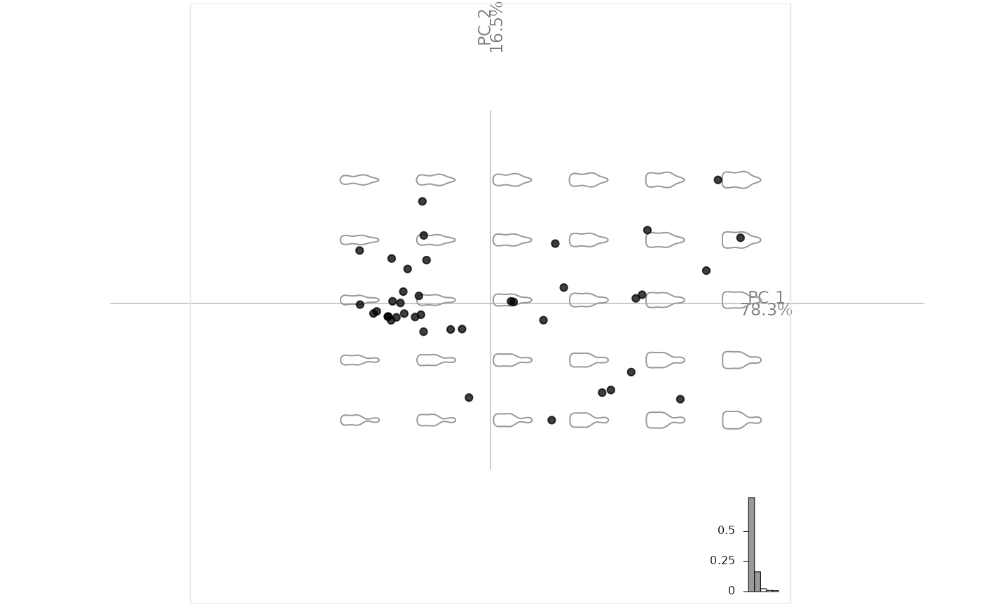
plot_PCA(bp)

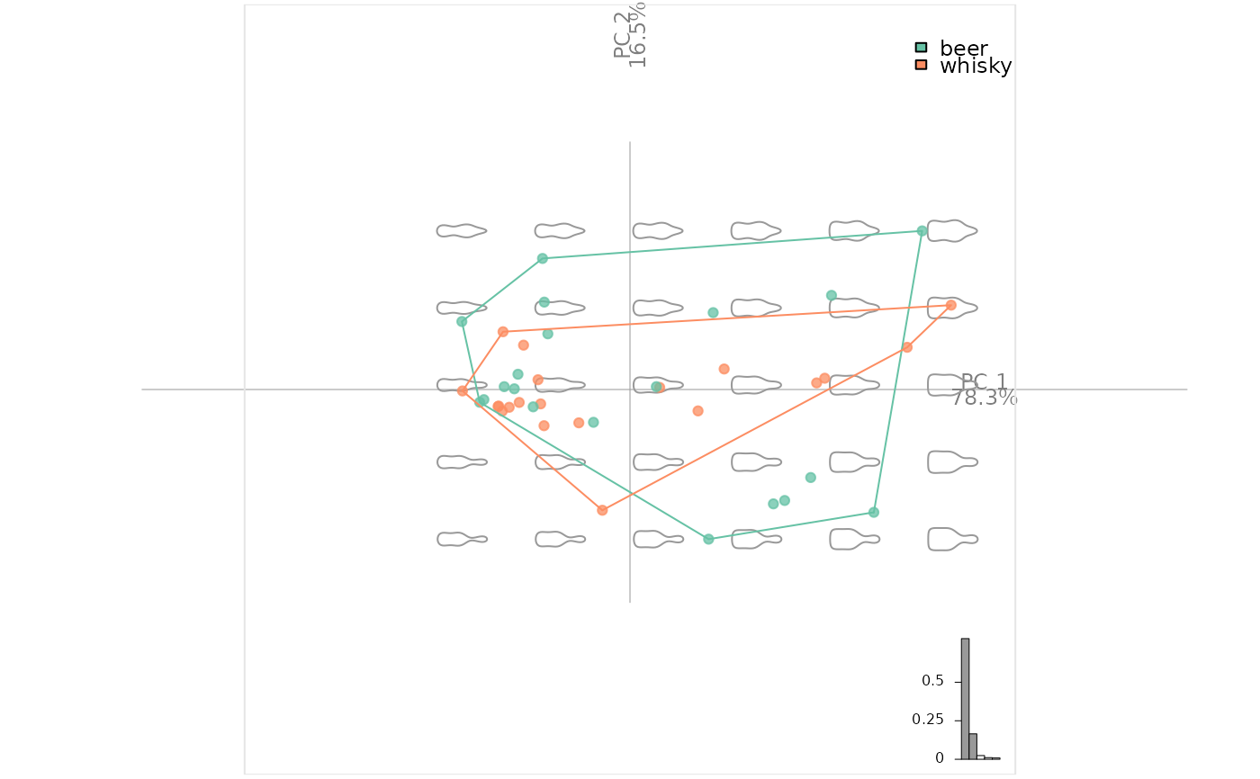
plot_PCA(bp, ~type)

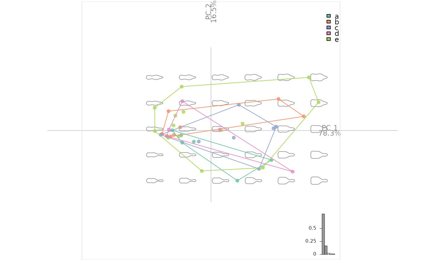
plot_PCA(bp, ~fake)
#> factor passed was a character, and coerced to a factor.


# Some curves with olea
op <- olea %>%
mutate(s=coo_area(.)) %>%
filter(var != "Cypre") %>%
chop(~view) %>% opoly(5, nb.pts=90) %>%
combine %>% PCA
op$fac$s %<>% as.character() %>% as.numeric()

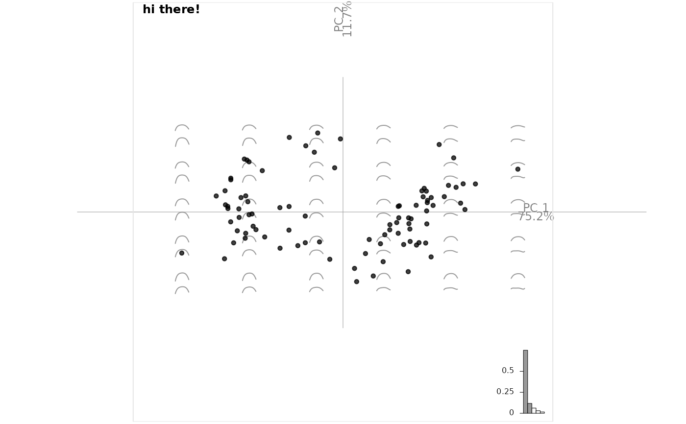
op %>% plot_PCA(title="hi there!")

### Now we can play with layers
# and for instance build a custom plot
# it should start with plot_PCA()

my_plot <- function(x, ...){

x %>%
    plot_PCA(...) %>%
    layer_points %>%
    layer_ellipsesaxes %>%
    layer_rug
}

# and even continue after this function
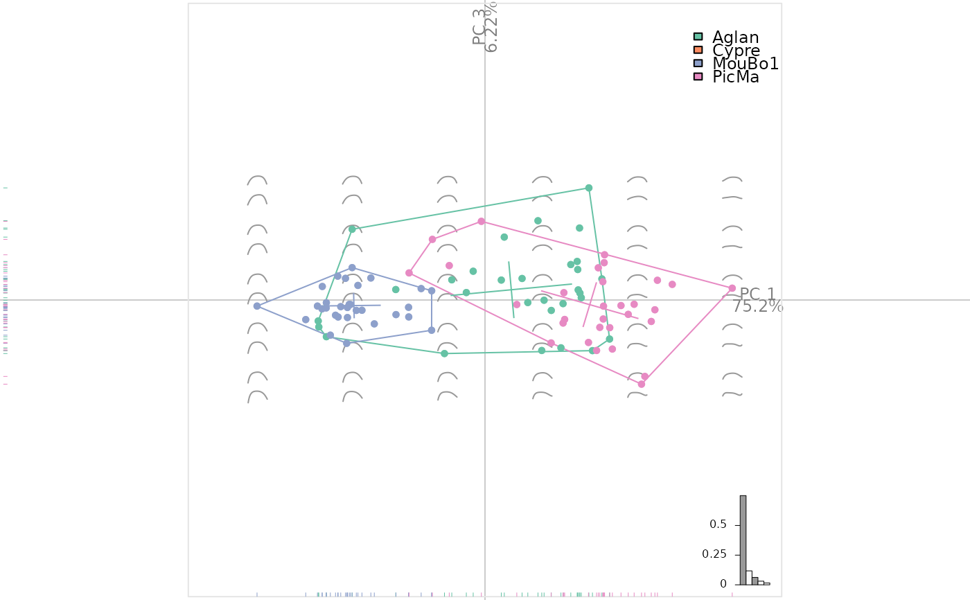
op %>% my_plot(~var, axes=c(1, 3)) %>%
    layer_title("hi there!")



# grindr allows (almost nice) tricks like highlighting:

# bp %>% .layerize_PCA(~fake) %>%
#   layer_frame %>% layer_axes() %>%
#   layer_morphospace_PCA() -> x

# highlight <- function(x, ..., col_F="#CCCCCC", col_T="#FC8D62FF"){
#  args <- list(...)
#  x$colors_groups <- c(col_F, col_T)
#  x$colors_rows <- c(col_F, col_T)[(x$f %in% args)+1]
#  x
#  }
# x %>% highlight("a", "b") %>% layer_points()

# You get the idea.