Preamble
In Momocs, a shape is a matrix of (x, y) coordinates. When they are plenty, they are usually gathered in a Coo object which is, essentially, a list with at least a $coo component.
## [1] TRUE## [,1] [,2]
## [1,] 37 561
## [2,] 40 540
## [3,] 40 529
## [4,] 43 508
## [5,] 46 487
## [6,] 48 477## [1] "Out" "Coo"## [1] TRUE## [1] "list"## $brahma
##      [,1] [,2]
## [1,]   37  561
## [2,]   40  540
## [3,]   40  529
## [4,]   43  508
## [5,]   46  487
## [6,]   48  477
##
## $caney
## [,1] [,2]
## [1,] 53 535
## [2,] 53 525
## [3,] 54 505
## [4,] 53 495
## [5,] 54 485
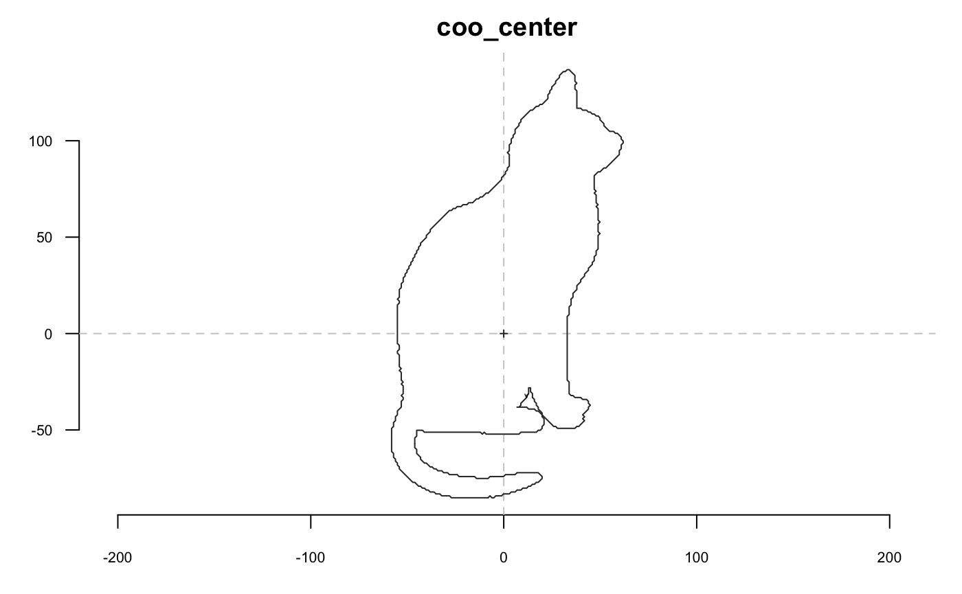
## [6,] 54 464Most operations on shapes can also be done on Coo objects. For example, getting the area or centering:
## [1] 234515## brahma caney chimay corona deusventrue duvel
## 234515.0 201056.5 119459.5 119568.5 165735.5 114015.0In other words most coo_ functions are actually methods that can actually be passed with a single matrix or a Coo object.
Below, we will distinguish coo_* operations based on whether they return a shape (eg if it is a geometric operation) or a scalar (a single number that can be used as a shape descriptor).
Not all are described but you can obtain a full list of coo_ operations with:
## [1] "coo_align"          "coo_aligncalliper"  "coo_alignminradius"
## [4] "coo_alignxax" "coo_angle_edges" "coo_angle_tangent"## [1] 95Scalar descriptors of shape
coo_scalar calculate all scalar descriptors included in Momocs. coo_rectilinearity is not included by default since it takes a looot of time to compute.
## # A tibble: 30 x 15
##      area calliper centsize circularity circularityharali… circularitynorm
##     <dbl>    <dbl>    <dbl>       <dbl>              <dbl>           <dbl>
##  1 20030.     319.     87.9        54.4               2.21            4.33
##  2 26078.     311.    103.         32.0               2.47            2.55
##  3 31516      280.     91.2        51.1               2.43            4.07
##  4 14180.     231.     73.0        46.6               2.84            3.71
##  5  9282.     206.     63.4        41.8               2.33            3.32
##  6 24060.     263.     91.2        35.9               3.84            2.85
##  7 14940.     263.     81.5        52.0               2.74            4.14
##  8 33921      352.    109.         35.7               2.83            2.84
##  9 18654      209.     67.3        74.1               2.45            5.89
## 10 36654.     312.     98.3       106.                2.72            8.45
## # ... with 20 more rows, and 9 more variables: convexity <dbl>,
## #   eccentricityboundingbox <dbl>, eccentricityeigen <dbl>,
## #   elongation <dbl>, length <dbl>, perim <dbl>, rectangularity <dbl>,
## #   solidity <dbl>, width <dbl>
Each of the function listed below has its own method that you can used by prefixing it with coo_; see the example below with coo_area.
## area
## calliper
## centsize
## circularity
## circularityharalick
## circularitynorm
## convexity
## eccentricityboundingbox
## eccentricityeigen
## elongation
## length
## perim
## rectangularity
## solidity
## width## [1] 14180.5## arrow bone buttefly cat check cross dog fish
## 20029.5 26078.5 31516.0 14180.5 9281.5 24060.5 14939.5 33921.0
## hand hands heart info lady leaf leaf2 leaf3
## 18654.0 36653.5 24276.5 8453.5 11541.0 12861.5 16993.5 18301.5
## leaf4 moon morph parrot penta pigeon plane puzzle
## 17748.5 13558.0 28292.0 7894.5 24709.0 23792.5 12649.0 16986.5
## rabbit sherrif snail star tetra umbrella
## 18915.5 15766.0 26992.5 23132.0 18119.0 16878.5## # A tibble: 6 x 2
## area perim
## <dbl> <dbl>
## 1 20030. 1044.
## 2 26078. 914.
## 3 31516 1269.
## 4 14180. 813.
## 5 9282. 623.
## 6 24060. 929.Geometric operations
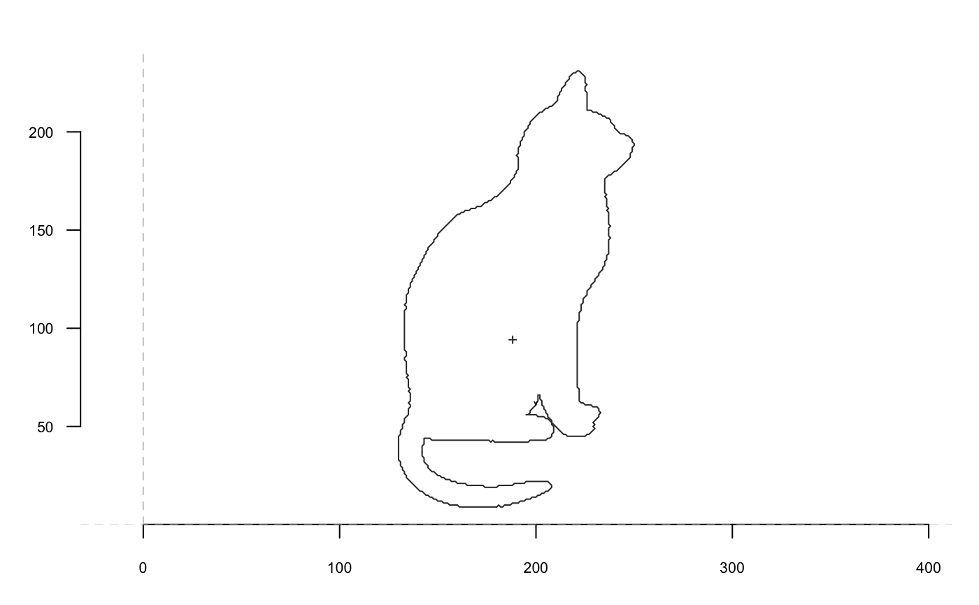
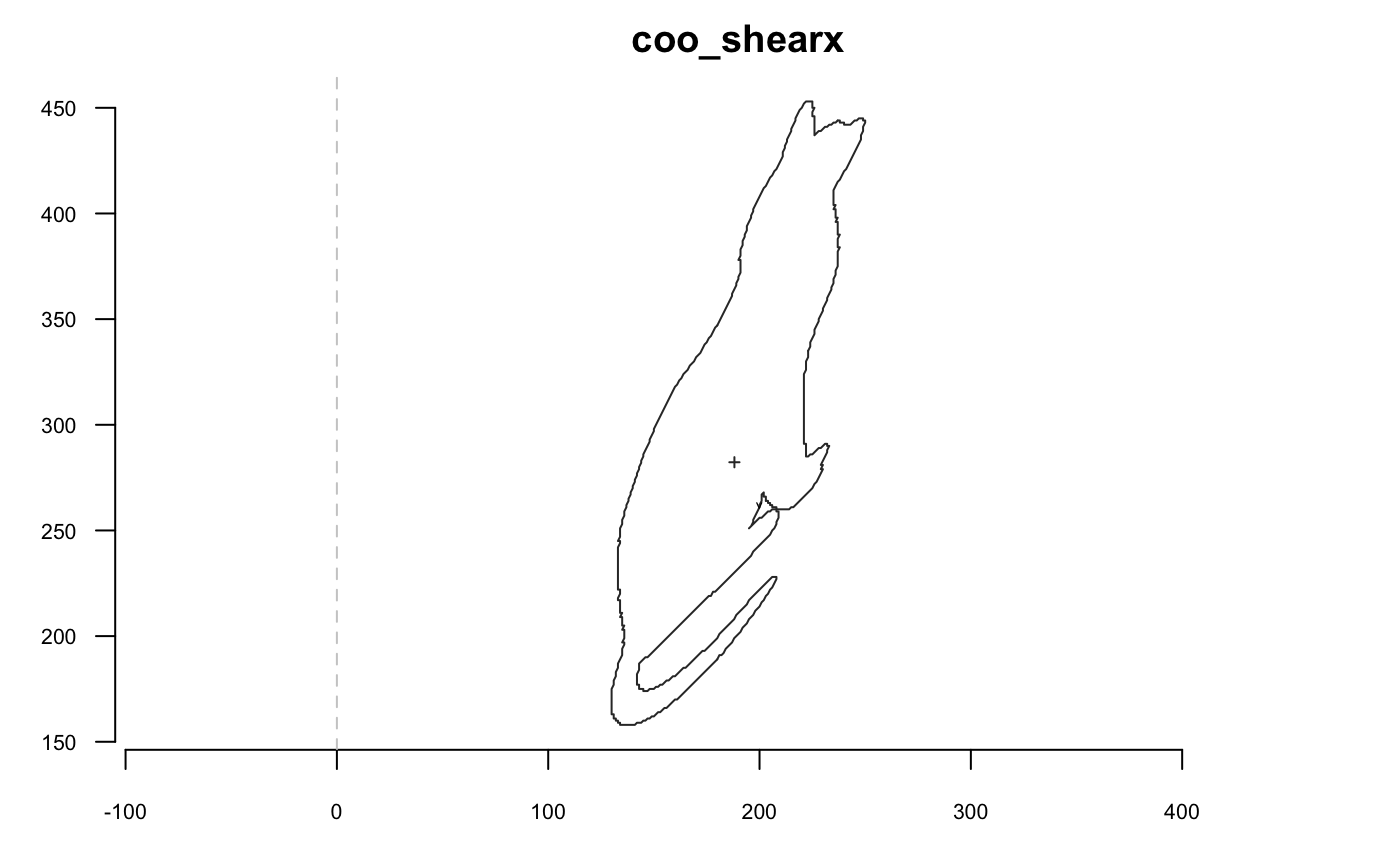
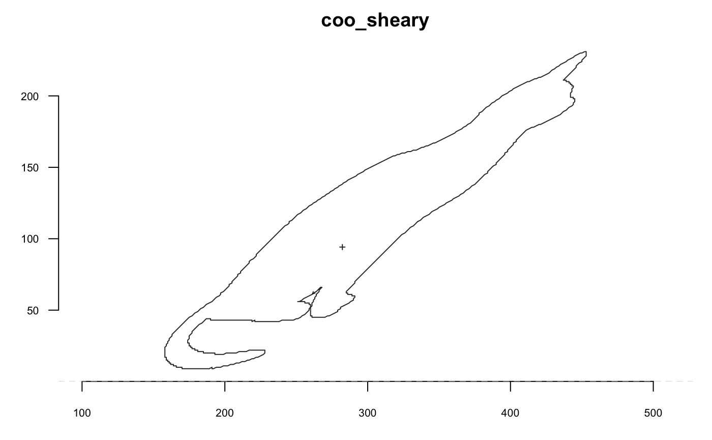
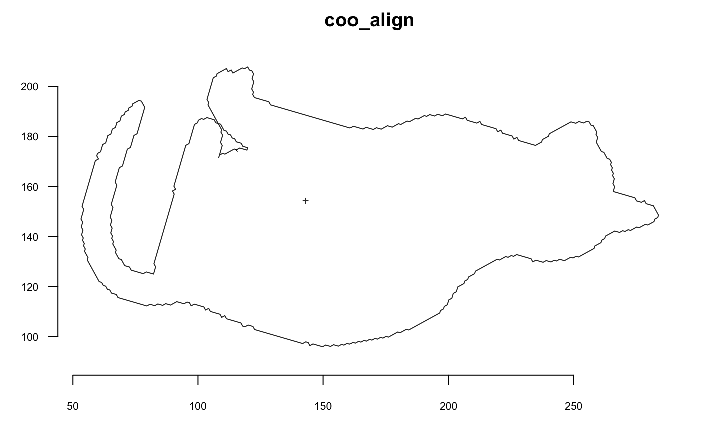
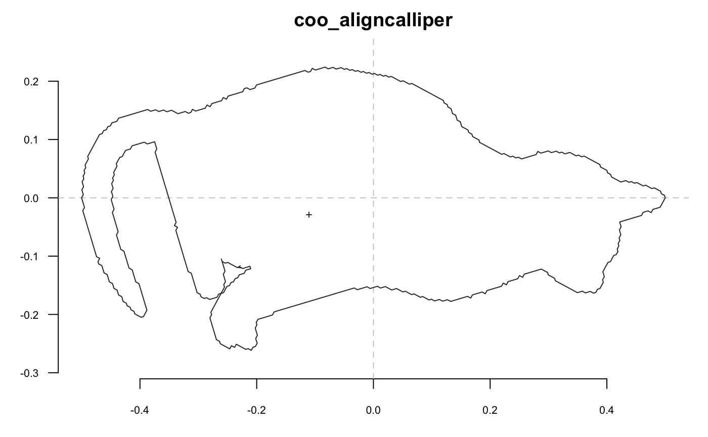
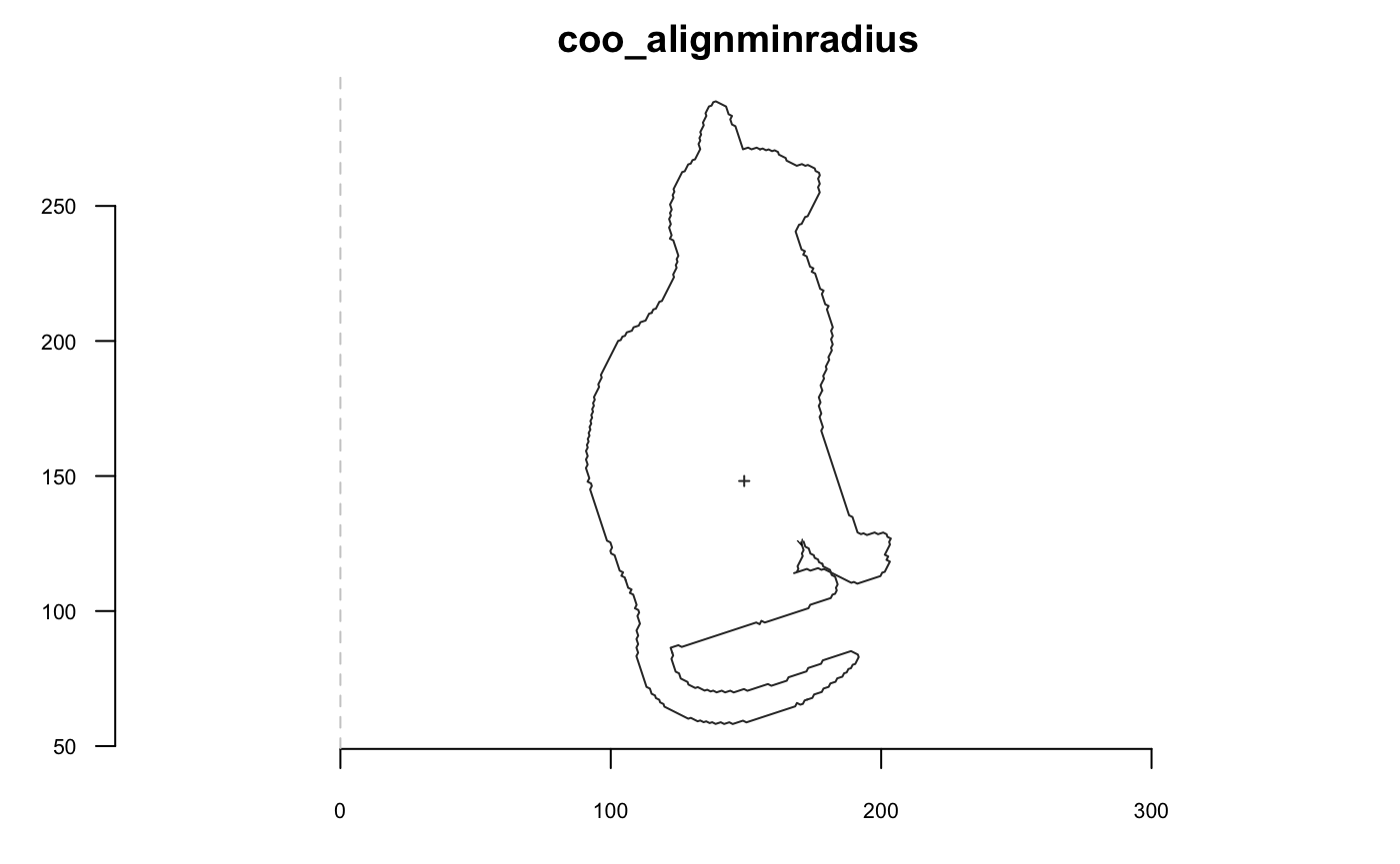
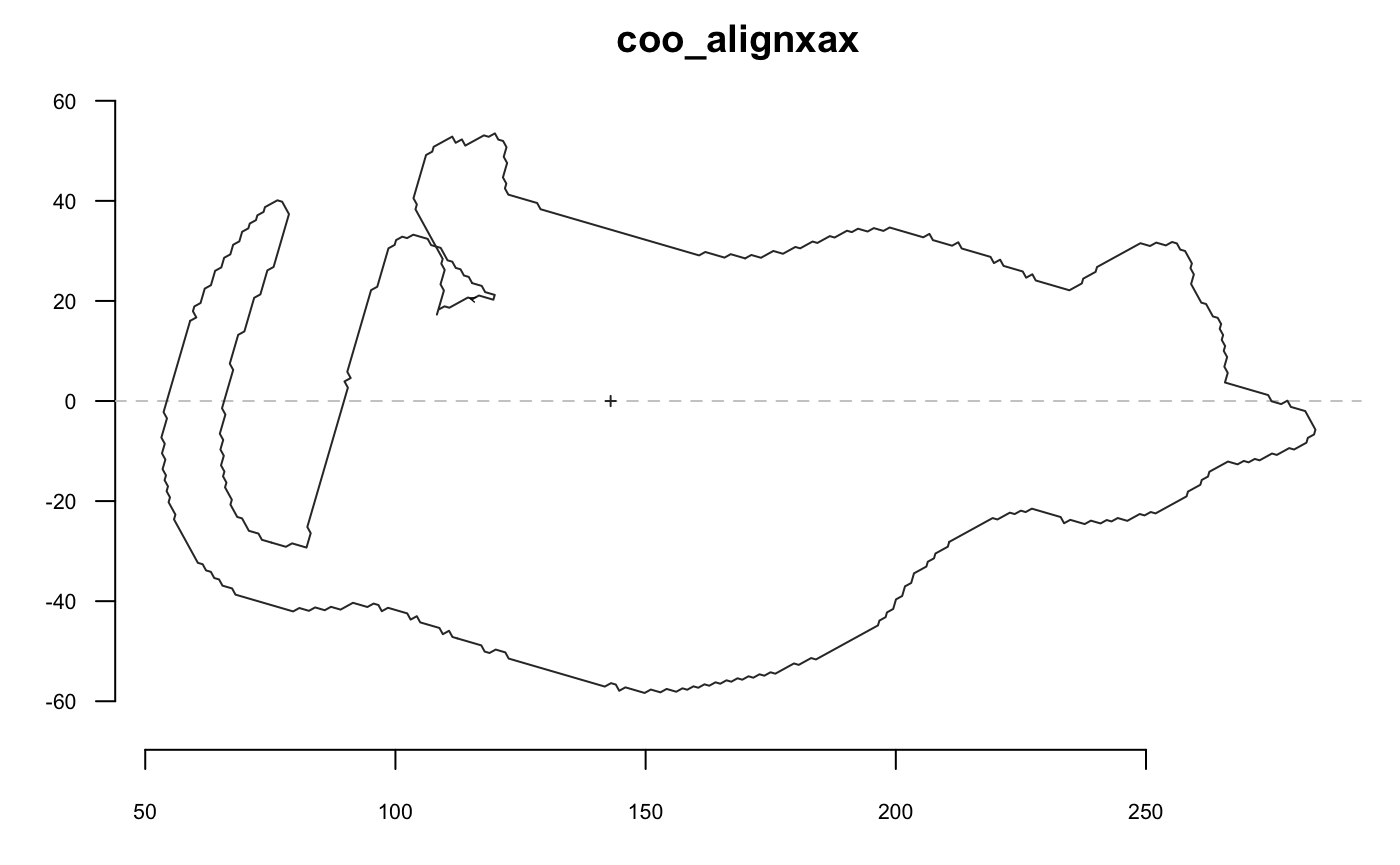
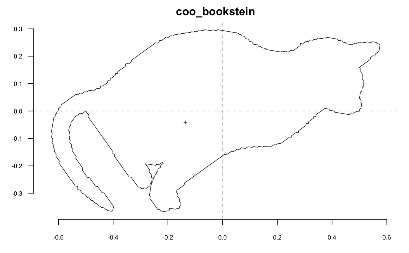
The functions below return shapes, so we exemplify them with graphs. For the sake of clarity/speed we illustrate them on single shape but, again, this can be done on Coo objects.
## will soon be deprecated, see ?pile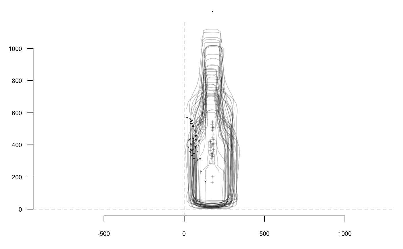
## will soon be deprecated, see ?pile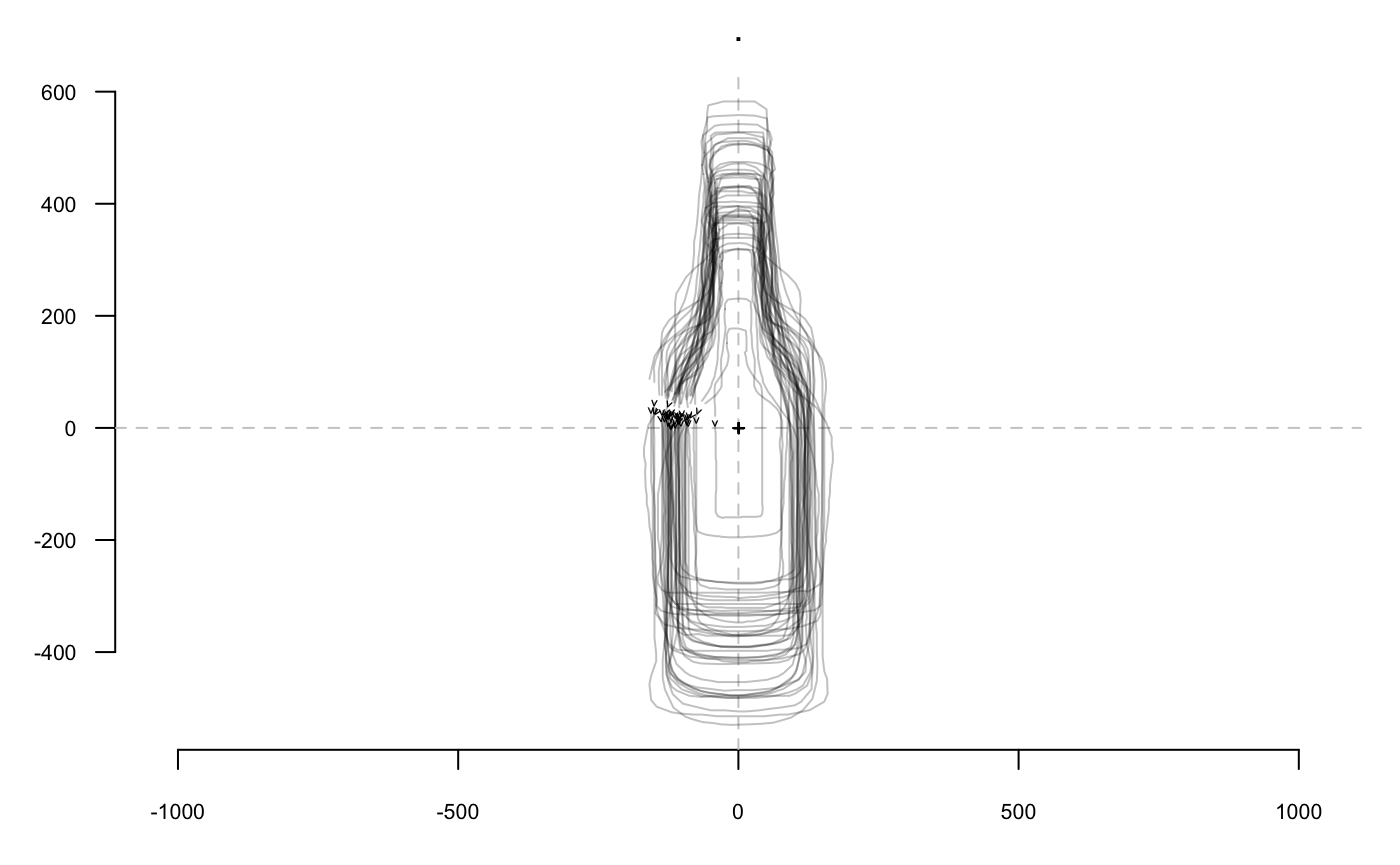
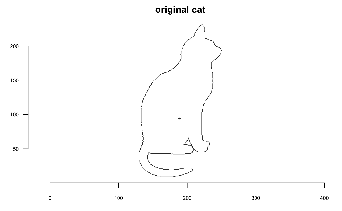
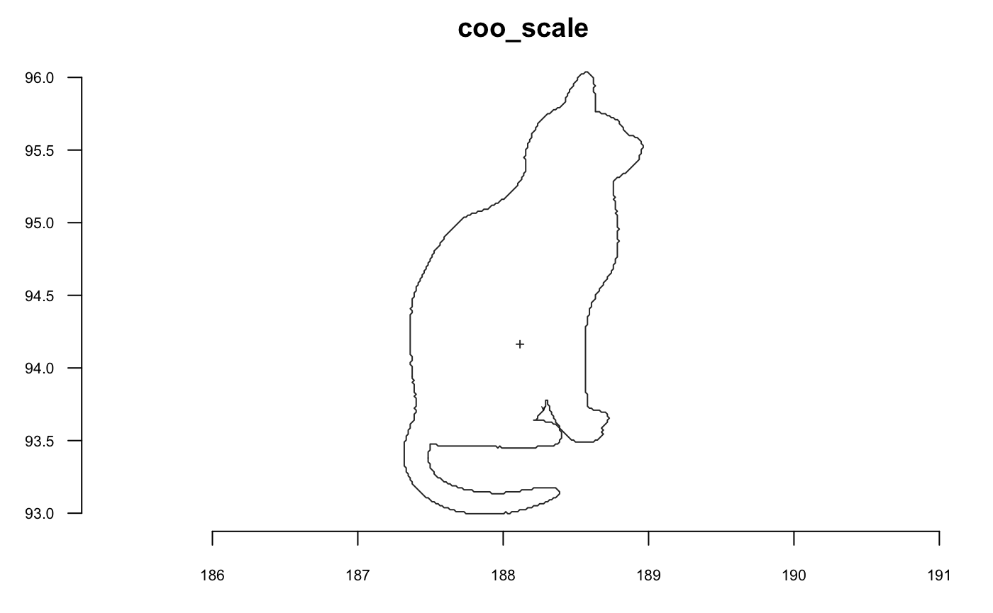
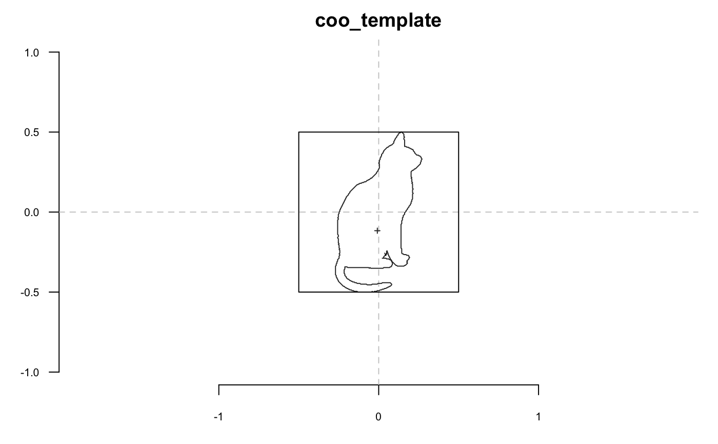
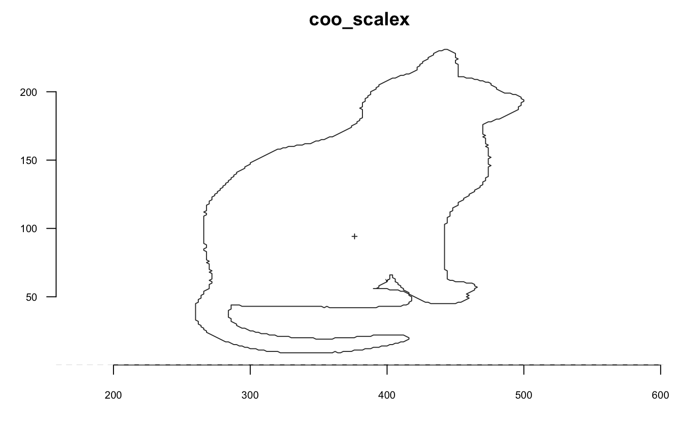
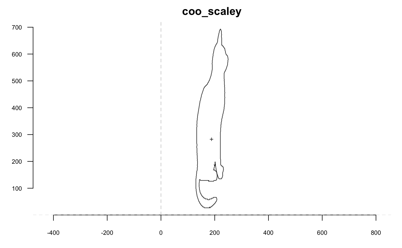
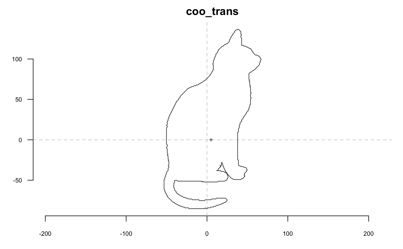
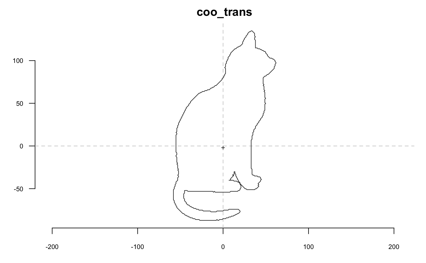
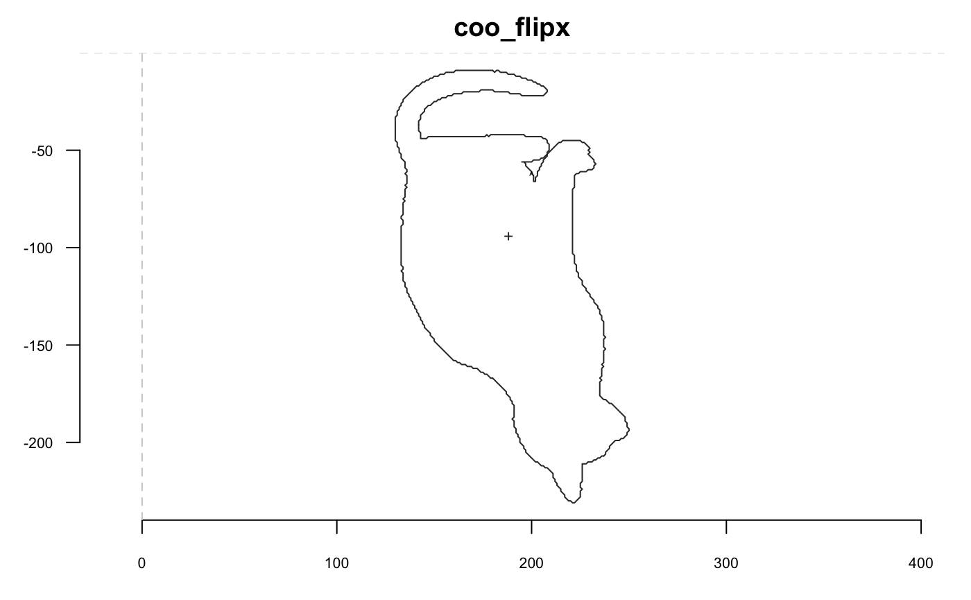
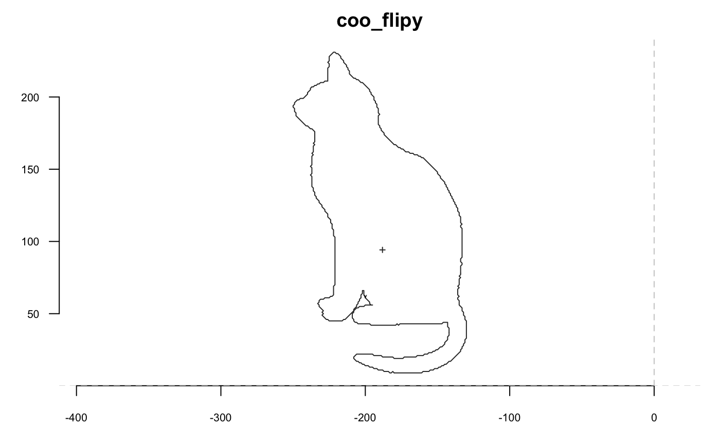
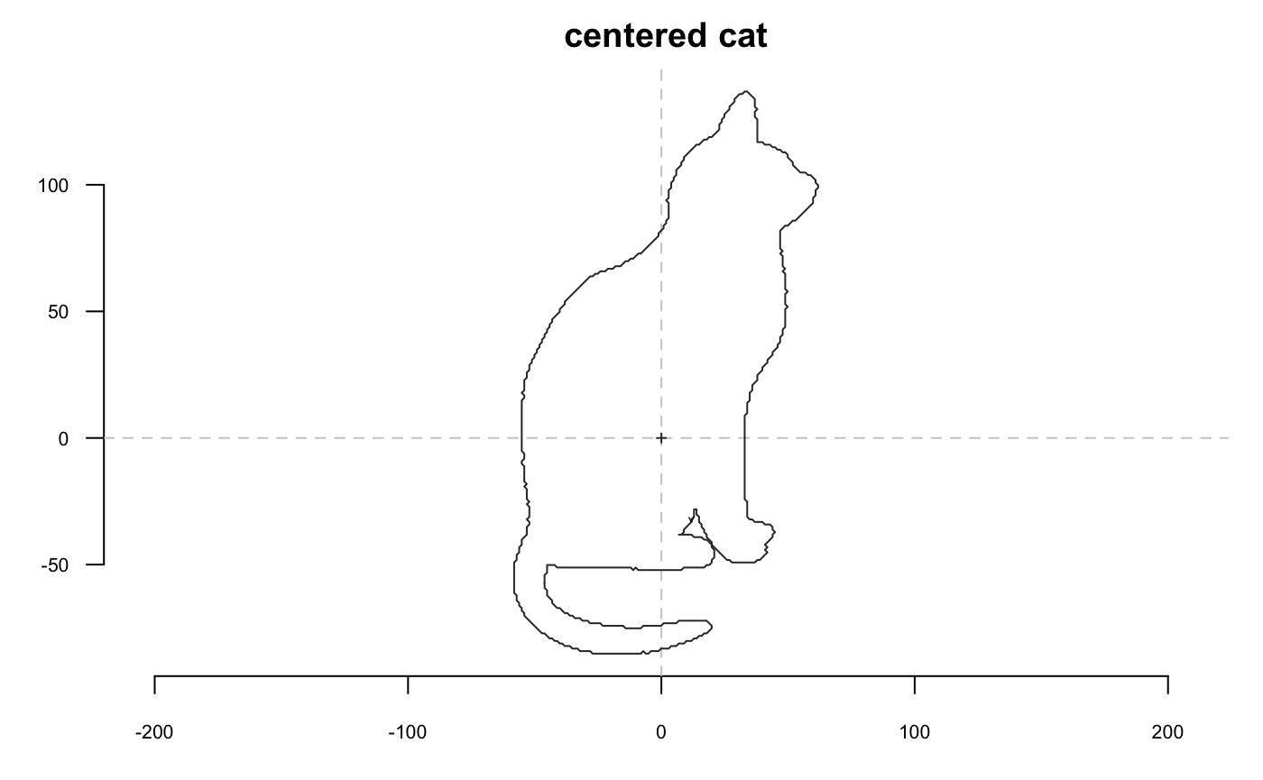
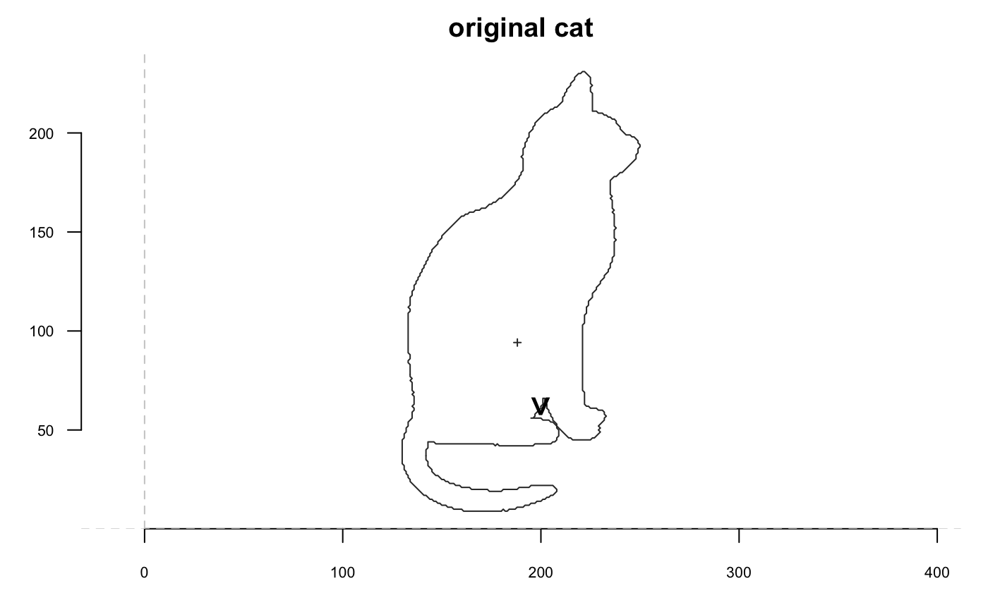
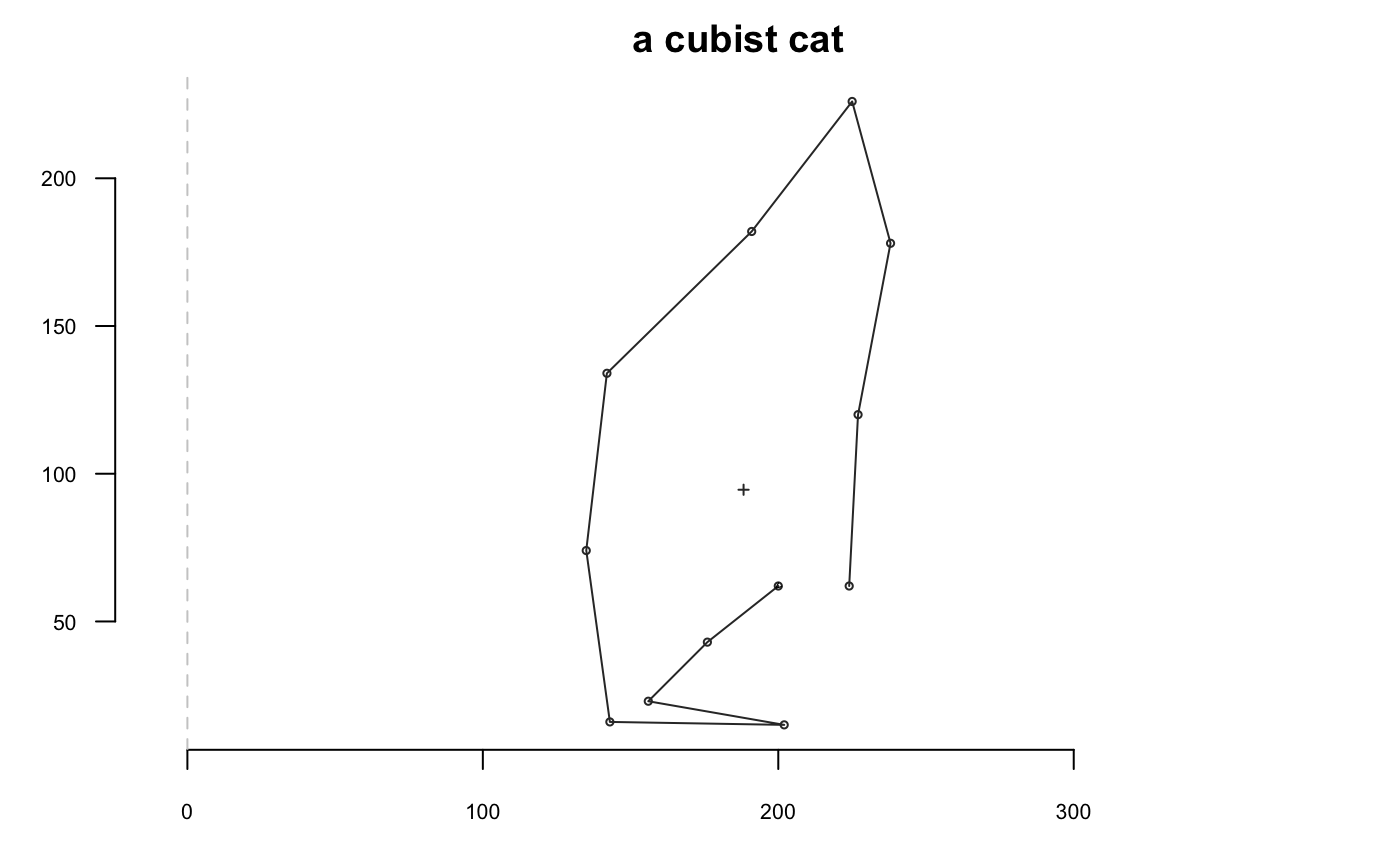
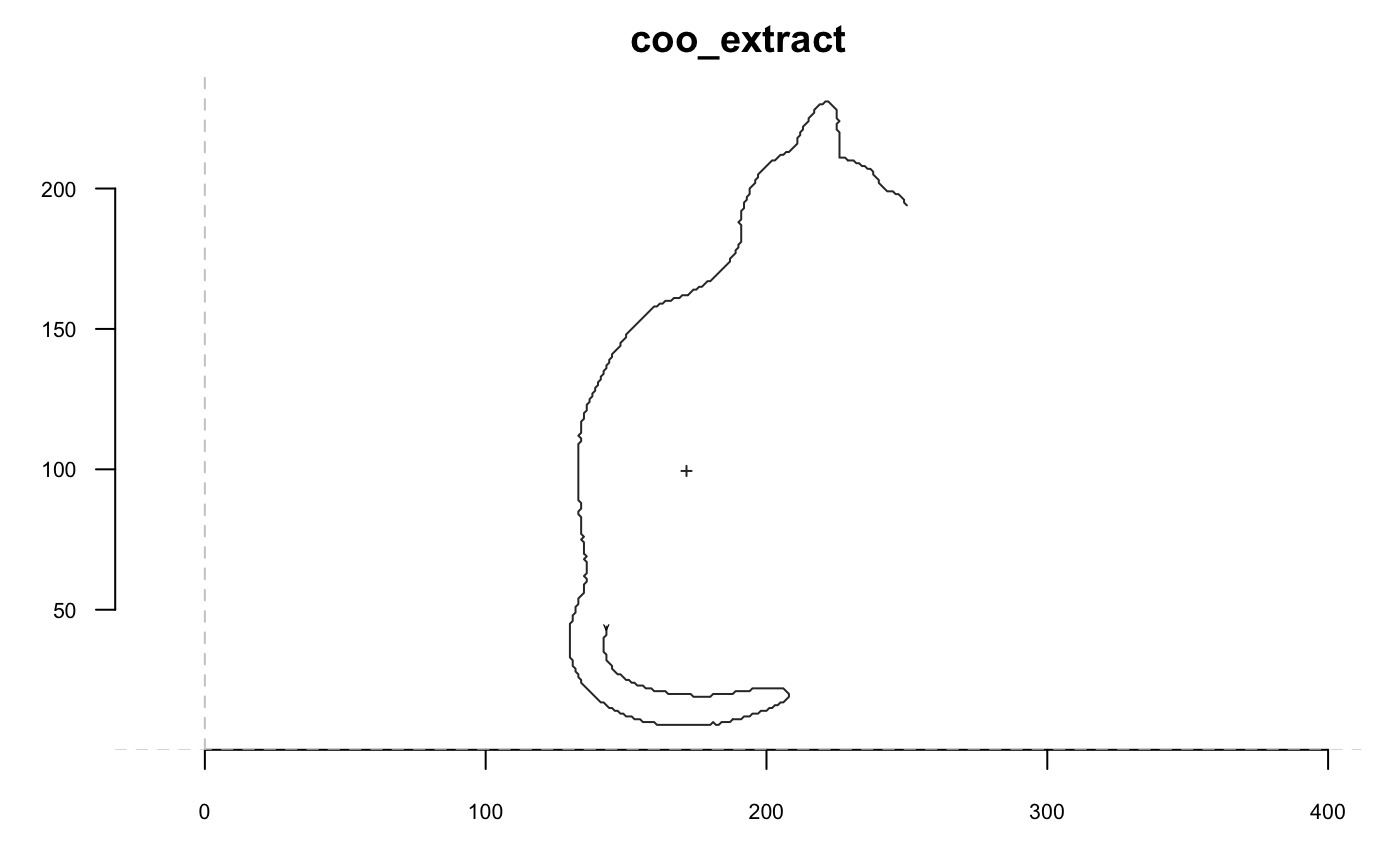
Now we go with a cat and we will extensively use coo_plot. We define a function that will help display side by side the original and transformed cat; when I use p(coo_align), it is equivalent to coo_align(your_shp) or shp %>% coo_align
Size
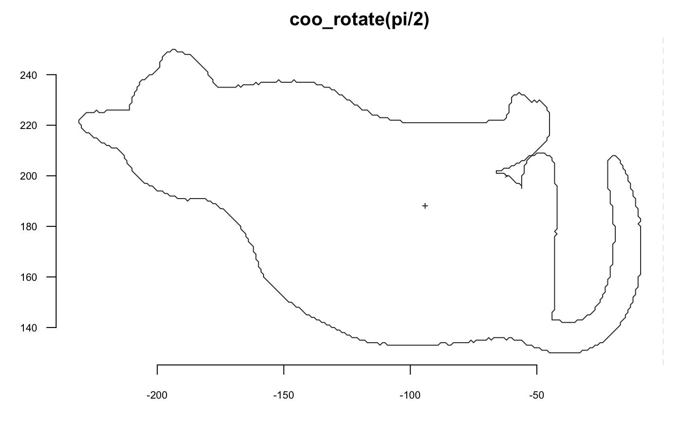
Rotation
shp %>% coo_rotatecenter(-pi/6, center=c(250, 195)) %>% coo_plot(main="coo_rotatecenter") # with center ~on cat's nose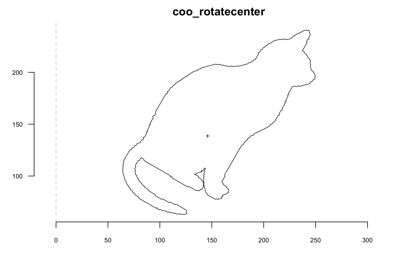
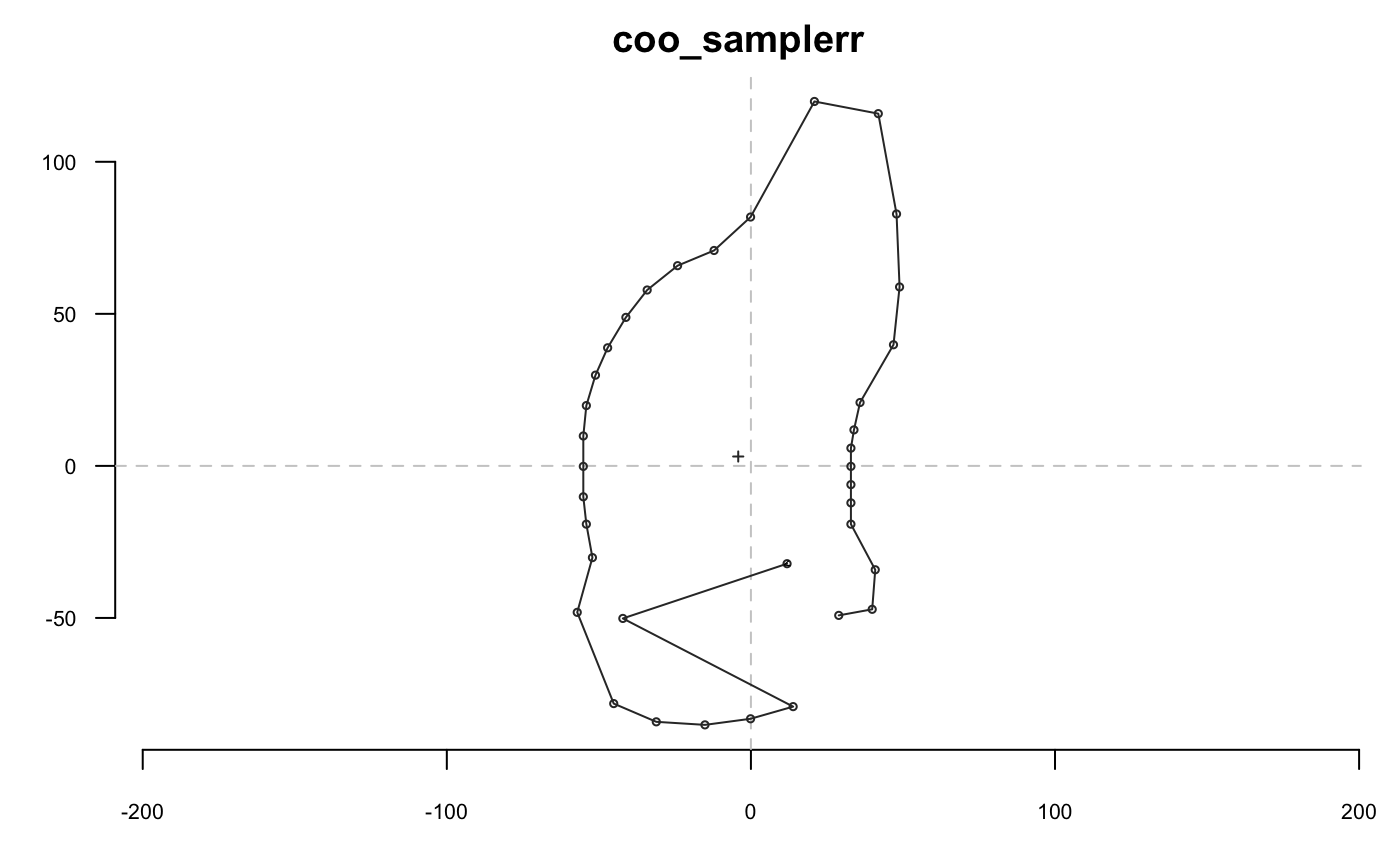
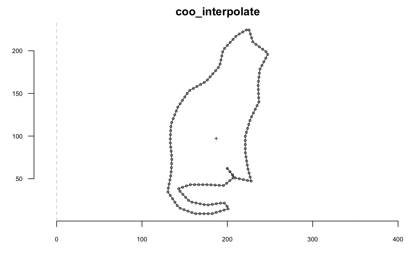
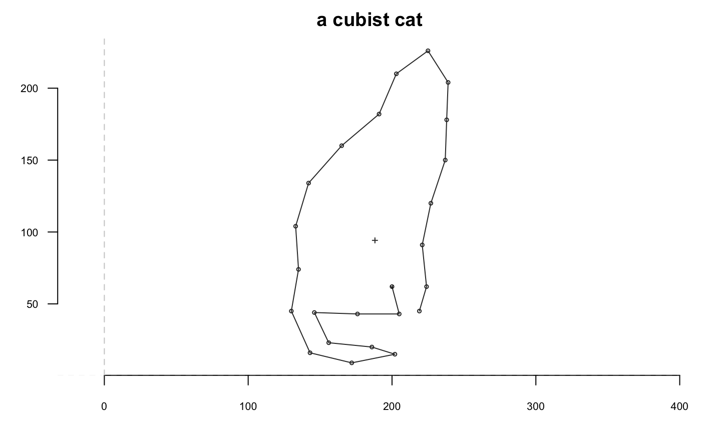
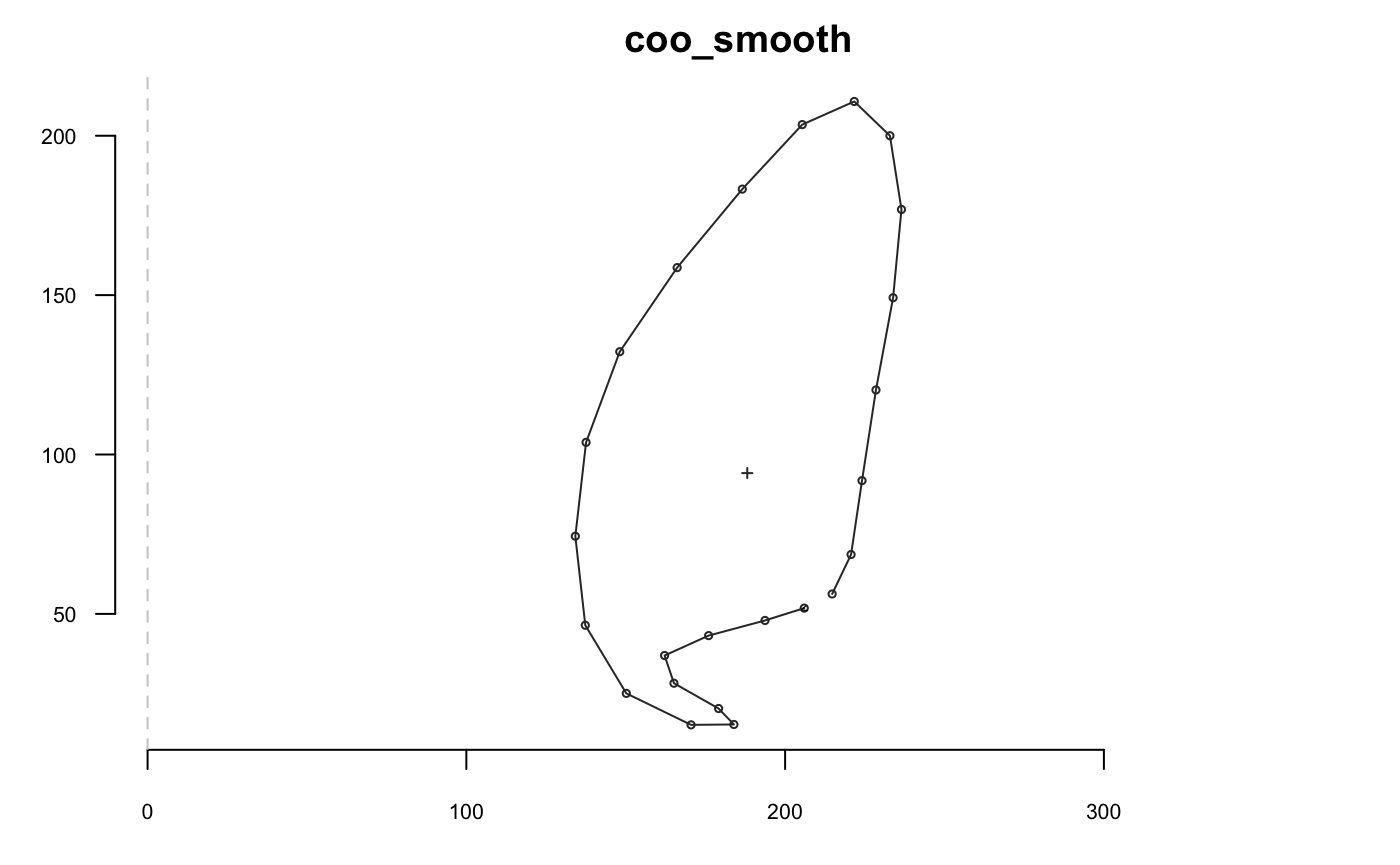
Sampling
## [1] 710shp %>% coo_sample(36) %>% coo_plot(main="coo_sample")
shp %>% coo_sample_prop(1/20) %>% coo_plot(main="coo_sample")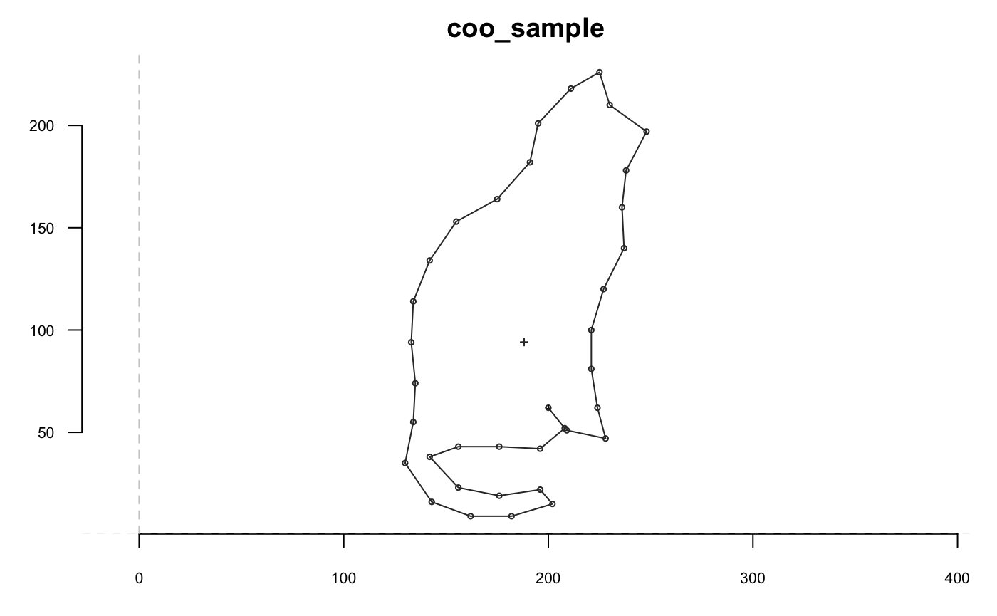
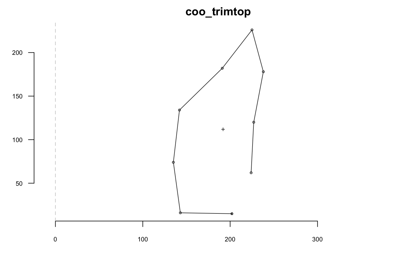
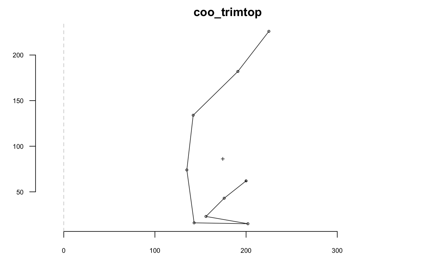
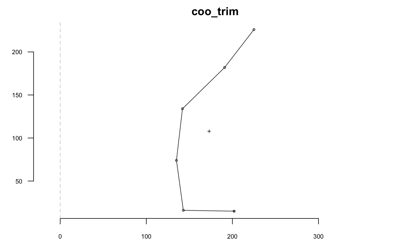
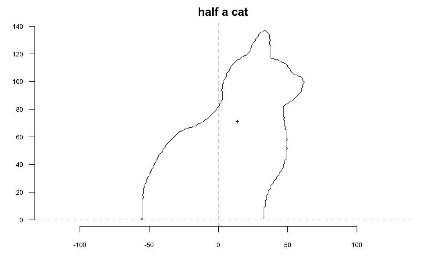
Slicing
Based on geometry
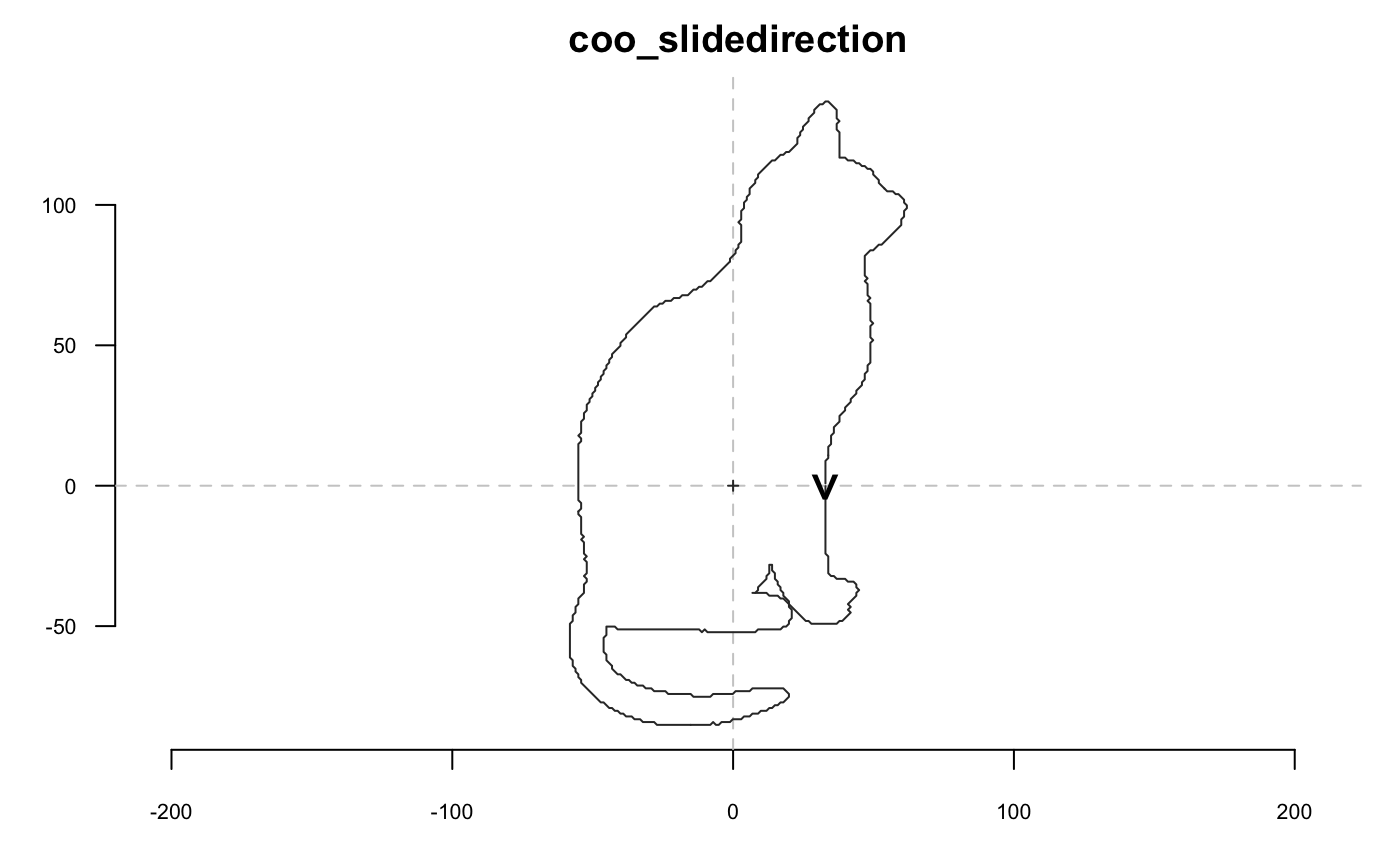
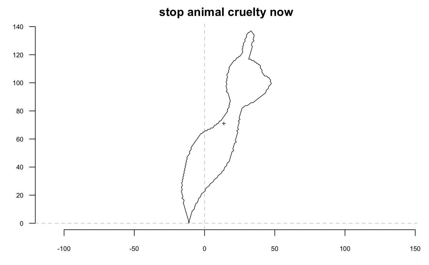
 If you want to slice but want the first point to be on one end, then
 coo_slidegap is your friend :
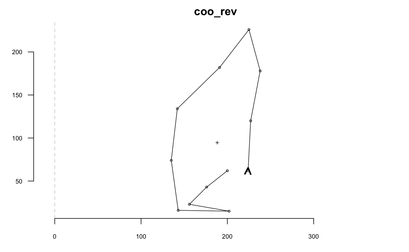
Indexing
Sliding
shp %>% coo_slide(id=93) %>% coo_plot(main="coo_slide", cex.first.point = 2) # same comment for ldk/Coo as for coo_slice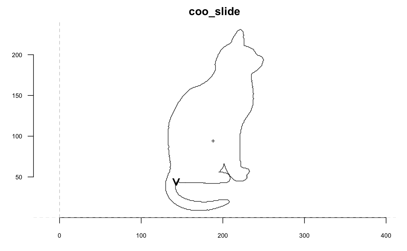
Misc
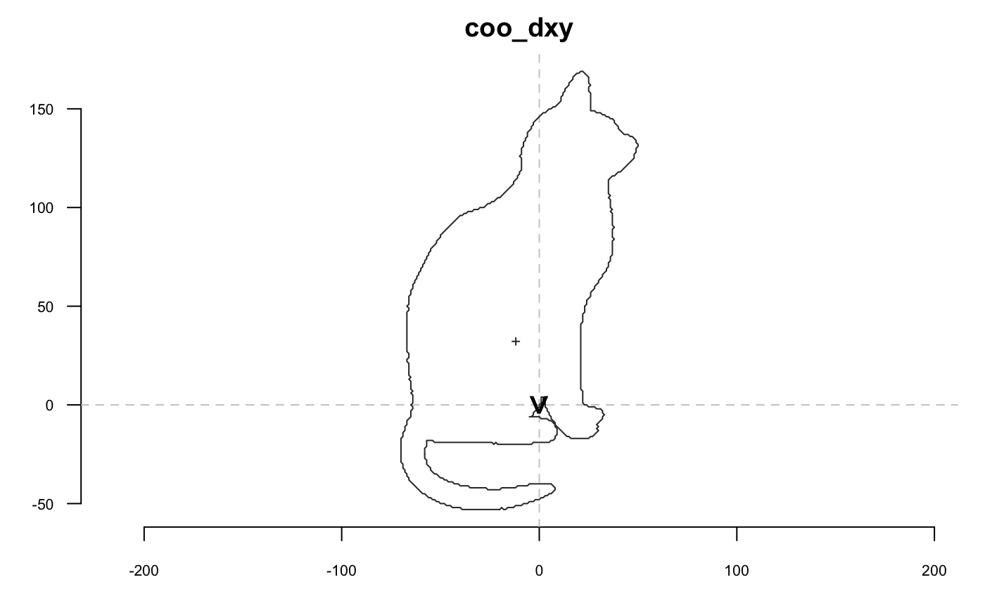
A side effect of coo_dxy is to set the first point on (0, 0)
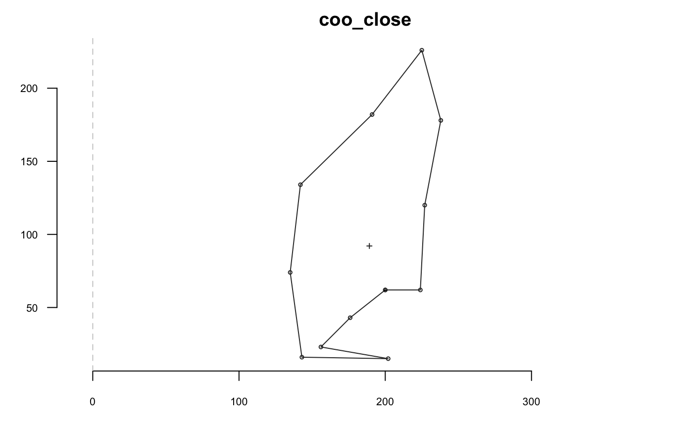
coo_force2close can be use to spread differences between the first and last point, and to force closing:
# for the sake of reproducibility
set.seed(123)
shp %>% coo_jitter(factor=10) %>% coo_plot(main="coo_jitter")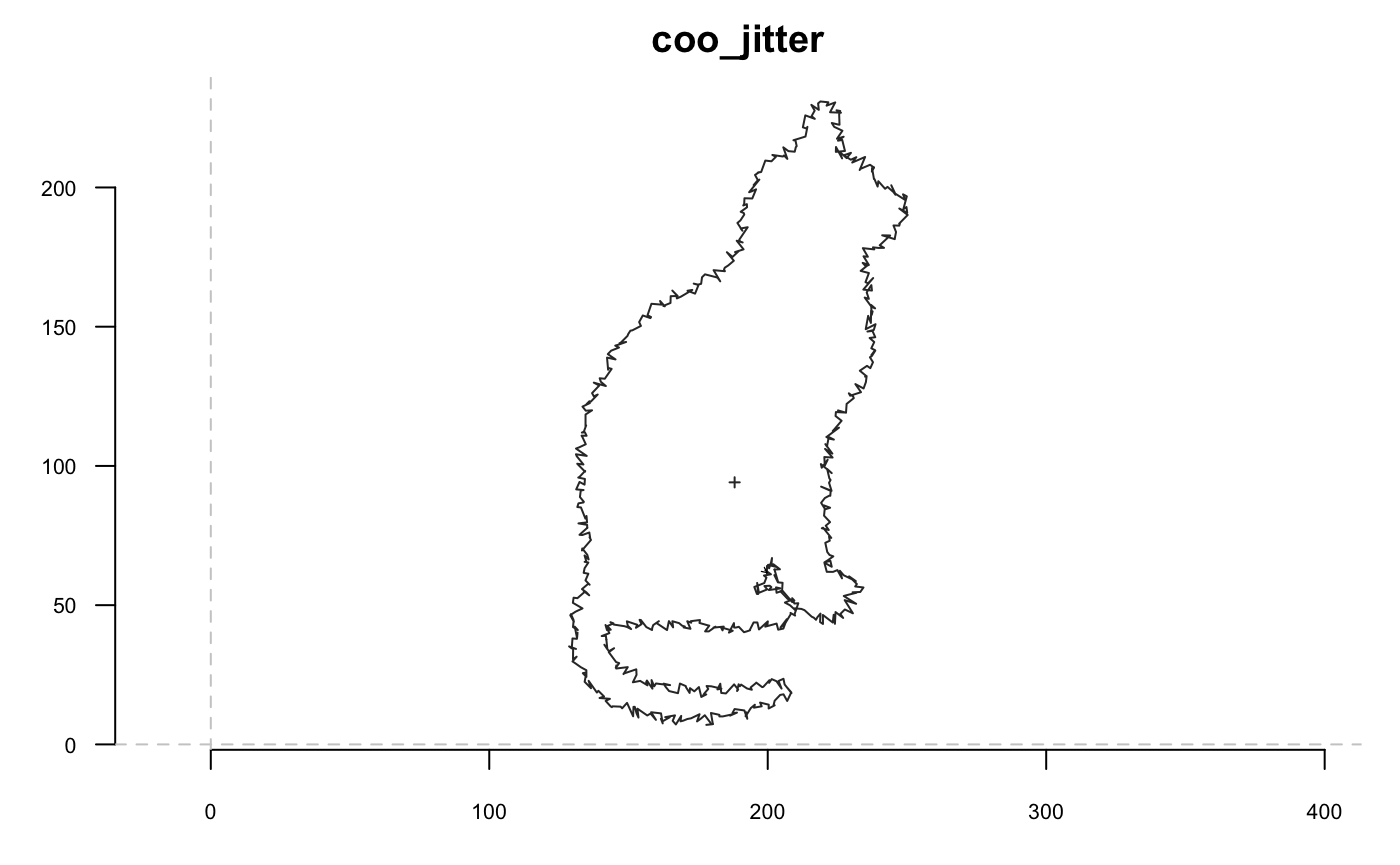
Other coo operations
# coo_descriptors along
coo_centdist
coo_perimcum
coo_perimpts


# coo_descriptors non-scalars
coo_boundingbox
coo_centpos # should be a df?
coo_chull
coo_chull_onion
coo_diffrange # coo_range_diff
coo_lw
coo_truss

coo_range
coo_range_enlarge

# coo_drawers
coo_arrows
coo_draw
coo_draw_rads
coo_listpanel
coo_lolli
coo_oscillo # deprecate for a proper oscillo
coo_plot
coo_ruban

# coo_others
coo_angle_edges
coo_angle_tangent

coo_intersect_angle
coo_intersect_direction
coo_intersect_segment

# coo_testers
coo_is_closed
coo_likely_anticlockwise
coo_likely_clockwise

# helpers
coo_check
coo_nb

coo_ldk