Calculate orthogonal polynomial fits on open outlines

Calculates orthogonal polynomial coefficients, through a linear model fit (see lm), from a matrix of (x; y) coordinates or a Opn object

Usage

opoly(x, ...)

# S3 method for default
opoly(x, degree, ...)

# S3 method for Opn
opoly(
  x,
  degree,
  baseline1 = c(-0.5, 0),
  baseline2 = c(0.5, 0),
  nb.pts = 120,
  ...
)

# S3 method for list
opoly(x, ...)

Arguments

x: a matrix (or a list) of (x; y) coordinates
...: useless here
degree: polynomial degree for the fit (the Intercept is also returned)
baseline1: numeric the \((x; y)\) coordinates of the first baseline by default \((x= -0.5; y=0)\)
baseline2: numeric the \((x; y)\) coordinates of the second baseline by default \((x= 0.5; y=0)\)
nb.pts: number of points to sample and on which to calculate polynomials

Value

a list with components when applied on a single shape:

coeff the coefficients (including the intercept)
ortho whether orthogonal or natural polynomials were fitted
degree degree of the fit (could be retrieved through coeff though)
baseline1 the first baseline point (so far the first point)
baseline2 the second baseline point (so far the last point)
r2 the r2 from the fit
mod the raw lm model

otherwise an OpnCoe object.

Note

Orthogonal polynomials are sometimes called Legendre's polynomials. They are preferred over natural polynomials since adding a degree do not change lower orders coefficients.

Examples

data(olea)
o <- olea[1]
op <- opoly(o, degree=4)
op
#> $coeff
#> (Intercept)          x1          x2          x3          x4 
#>  0.20937101  0.01991936 -0.95319289 -0.03075138 -0.11975200 
#> 
#> $ortho
#> [1] TRUE
#> 
#> $degree
#> [1] 4
#> 
#> $baseline1
#> [1] -0.5  0.0
#> 
#> $baseline2
#> [1] 0.5 0.0
#> 
#> $r2
#> [1] 0.9986415
#> 
#> $mod
#> 
#> Call:
#> lm(formula = coo[, 2] ~ x)
#> 
#> Coefficients:
#> (Intercept)           x1           x2           x3           x4  
#>     0.20937      0.01992     -0.95319     -0.03075     -0.11975  
#> 
#> 
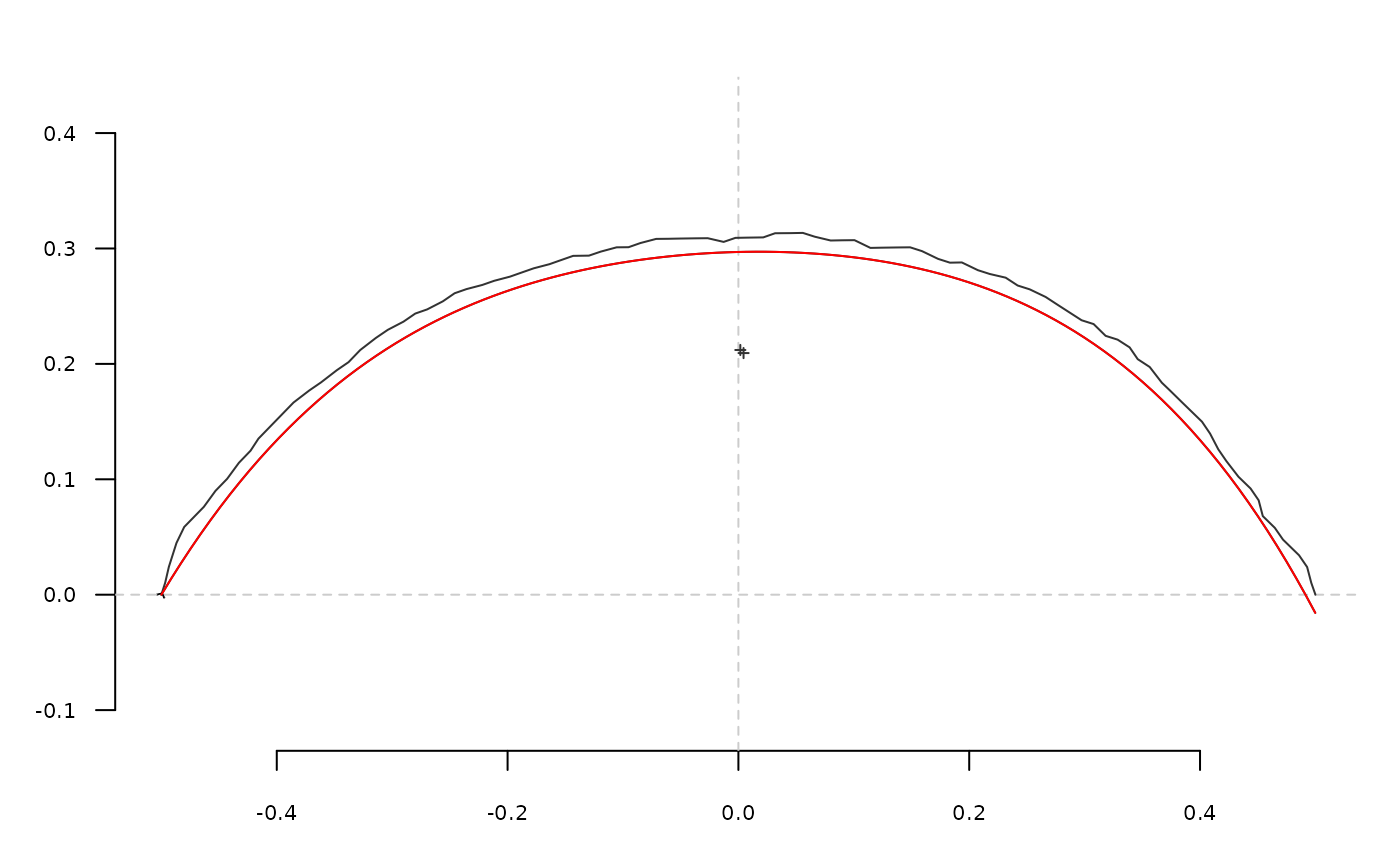
# shape reconstruction
opi <- opoly_i(op)
coo_plot(o)
coo_draw(opi)
lines(opi, col='red')

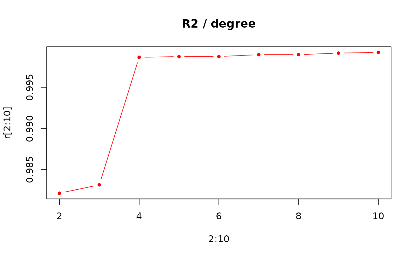
# R2 for degree 1 to 10
r <- numeric()
for (i in 1:10) { r[i] <- opoly(o, degree=i)$r2 }
plot(2:10, r[2:10], type='b', pch=20, col='red', main='R2 / degree')