In Momocs, Opn classes objects are
lists of open outlines, with optionnal components,
on which generic methods such as plotting methods (e.g. stack)
and specific methods (e.g. npoly can be applied.
Opn objects are primarily Coo objects.
Examples
#Methods on Opn
methods(class=Opn)
#> [1] add_ldk combine coo_bookstein coo_sample
#> [5] coo_sample_prop coo_slice coo_smoothcurve def_ldk
#> [9] def_ldk_angle def_ldk_direction def_ldk_tips dfourier
#> [13] fgProcrustes get_ldk mosaic npoly
#> [17] opoly panel pile rearrange_ldk
#> see '?methods' for accessing help and source code
# we load some open outlines. See ?olea for credits
olea
#> Opn (curves)
#> - 210 curves, 99 +/- 3 coords (in $coo)
#> - 4 classifiers (in $fac):
#> # A tibble: 210 × 4
#> var domes view ind
#> <fct> <fct> <fct> <fct>
#> 1 Aglan cult VD O10
#> 2 Aglan cult VL O10
#> 3 Aglan cult VD O11
#> 4 Aglan cult VL O11
#> 5 Aglan cult VD O12
#> 6 Aglan cult VL O12
#> # ℹ 204 more rows
#> - also: $ldk
panel(olea)
 # orthogonal polynomials
op <- opoly(olea, degree=5)
#> 'nb.pts' missing and set to 91
# we print the Coe
op
#> An OpnCoe object [ opoly analysis ]
#> --------------------
#> - $coe: 210 open outlines described
#> - $baseline1: (-0.5; 0), $baseline2: (0.5; 0)
#> # A tibble: 210 × 4
#> var domes view ind
#> <fct> <fct> <fct> <fct>
#> 1 Aglan cult VD O10
#> 2 Aglan cult VL O10
#> 3 Aglan cult VD O11
#> 4 Aglan cult VL O11
#> 5 Aglan cult VD O12
#> 6 Aglan cult VL O12
#> # ℹ 204 more rows
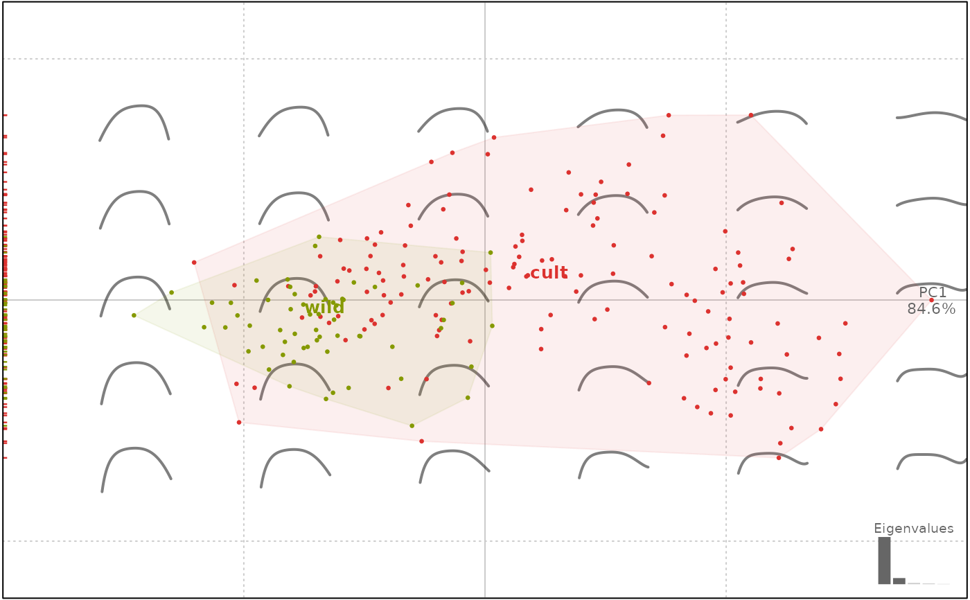
# Let's do a PCA on it
op.p <- PCA(op)
plot(op.p, 'domes')
#> will be deprecated soon, see ?plot_PCA
# orthogonal polynomials
op <- opoly(olea, degree=5)
#> 'nb.pts' missing and set to 91
# we print the Coe
op
#> An OpnCoe object [ opoly analysis ]
#> --------------------
#> - $coe: 210 open outlines described
#> - $baseline1: (-0.5; 0), $baseline2: (0.5; 0)
#> # A tibble: 210 × 4
#> var domes view ind
#> <fct> <fct> <fct> <fct>
#> 1 Aglan cult VD O10
#> 2 Aglan cult VL O10
#> 3 Aglan cult VD O11
#> 4 Aglan cult VL O11
#> 5 Aglan cult VD O12
#> 6 Aglan cult VL O12
#> # ℹ 204 more rows
# Let's do a PCA on it
op.p <- PCA(op)
plot(op.p, 'domes')
#> will be deprecated soon, see ?plot_PCA
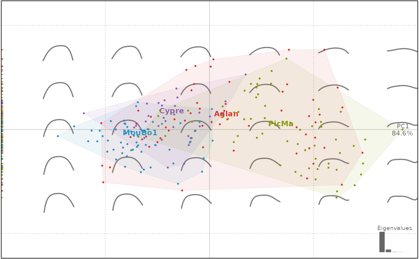
 plot(op.p, 'var')
#> will be deprecated soon, see ?plot_PCA
plot(op.p, 'var')
#> will be deprecated soon, see ?plot_PCA
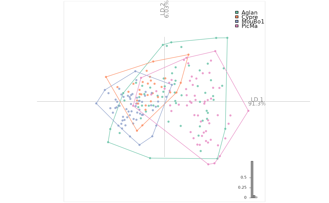
 # and now an LDA after a PCA
olda <- LDA(PCA(op), 'var')
#> 4 PC retained
# for CV table and others
olda
#> * Cross-validation table ($CV.tab):
#> classified
#> actual Aglan Cypre MouBo1 PicMa
#> Aglan 21 2 17 20
#> Cypre 12 4 14 0
#> MouBo1 4 2 54 0
#> PicMa 22 1 2 35
#>
#> * Class accuracy ($CV.ce):
#> Aglan Cypre MouBo1 PicMa
#> 0.3500000 0.1333333 0.9000000 0.5833333
#>
#> * Leave-one-out cross-validation ($CV.correct): (54.3% - 114/210):
plot_LDA(olda)
# and now an LDA after a PCA
olda <- LDA(PCA(op), 'var')
#> 4 PC retained
# for CV table and others
olda
#> * Cross-validation table ($CV.tab):
#> classified
#> actual Aglan Cypre MouBo1 PicMa
#> Aglan 21 2 17 20
#> Cypre 12 4 14 0
#> MouBo1 4 2 54 0
#> PicMa 22 1 2 35
#>
#> * Class accuracy ($CV.ce):
#> Aglan Cypre MouBo1 PicMa
#> 0.3500000 0.1333333 0.9000000 0.5833333
#>
#> * Leave-one-out cross-validation ($CV.correct): (54.3% - 114/210):
plot_LDA(olda)