LDA plot using grindr layers

Quickly vizualise LDA objects and build customs plots using the layers. See examples.

Usage

plot_LDA(
  x,
  axes = c(1, 2),
  palette = pal_qual,
  points = TRUE,
  points_transp = 1/4,
  morphospace = FALSE,
  morphospace_position = "range",
  chull = TRUE,
  chullfilled = FALSE,
  labelgroups = FALSE,
  legend = TRUE,
  title = "",
  center_origin = TRUE,
  zoom = 0.9,
  eigen = TRUE,
  box = TRUE,
  iftwo_layer = layer_histogram_2,
  iftwo_split = FALSE,
  axesnames = TRUE,
  axesvar = TRUE
)

Arguments

x

LDA object

axes

numeric of length two to select PCs to use (c(1, 2) by default)

palette

color palette to use col_summer by default

points

logical whether to draw this with layer_points

points_transp

numeric to feed layer_points (default:0.25)

morphospace

logical whether to draw this using layer_morphospace_PCA

morphospace_position

to feed layer_morphospace_PCA (default: "range")

chull

logical whether to draw this with layer_chull

chullfilled

logical whether to draw this with layer_chullfilled

labelgroups

logical whether to draw this with layer_labelgroups

legend

logical whether to draw this with layer_legend

title

character if specified, fee layer_title (default to "")

center_origin

logical whether to center origin

zoom

numeric zoom level for the frame (default: 0.9)

eigen

logical whether to draw this using layer_eigen

box

logical whether to draw this using layer_box

iftwo_layer

function (no quotes) for drawing LD1 when there are two levels. So far, one of layer_histogram_2 (default) or layer_density_2

iftwo_split

to feed split argument in layer_histogram_2 or layer_density_2

axesnames

logical whether to draw this using layer_axesnames

axesvar

logical whether to draw this using layer_axesvar

Value

a plot

Note

This approach will replace plot.LDA. This is part of grindr approach that may be packaged at some point. All comments are welcome.

See also

Other grindr: drawers, layers_morphospace, layers, mosaic_engine(), papers, pile(), plot_NMDS(), plot_PCA()

Examples

### First prepare an LDA object

# Some outlines with bot
bl <- bot %>%
      # cheap alignement before efourier
      coo_align() %>% coo_center %>% coo_slidedirection("left") %>%
      # add a fake column
      mutate(fake=sample(letters[1:5], 40, replace=TRUE)) %>%
      # EFT
      efourier(6, norm=FALSE) %>%
      # LDA
      LDA(~fake)
#> factor passed was a character, and coerced to a factor.

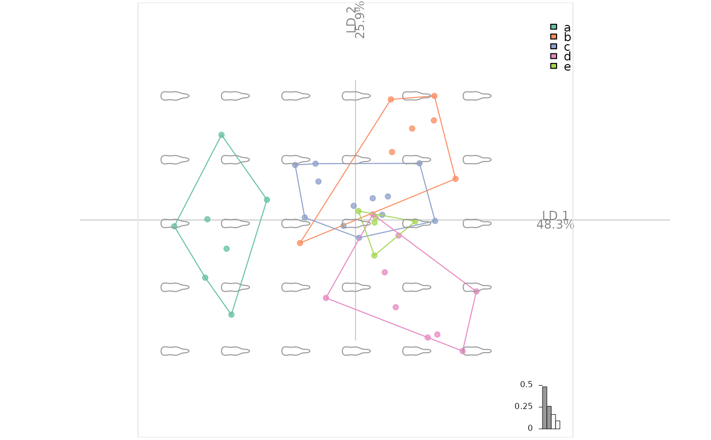
bl %>% plot_LDA %>% layer_morphospace_LDA
#> * layer_morphospace_LDA is back, but experimental


# Below inherited from plot_PCA and to adapt here.
#plot_PCA(bp)
#plot_PCA(bp, ~type)
#plot_PCA(bp, ~fake)

# Some curves with olea
#op <- olea %>%
#mutate(s=coo_area(.)) %>%
#filter(var != "Cypre") %>%
#chop(~view) %>% lapply(opoly, 5, nb.pts=90) %>%
#combine %>% PCA
#op$fac$s %<>% as.character() %>% as.numeric()

#op %>% plot_PCA(title="hi there!")

### Now we can play with layers
# and for instance build a custom plot
# it should start with plot_PCA()

#my_plot <- function(x, ...){

#x %>%
#     plot_PCA(...) %>%
#    layer_points %>%
#     layer_ellipsesaxes %>%
#    layer_rug
# }

# and even continue after this function
# op %>% my_plot(~var, axes=c(1, 3)) %>%
#     layer_title("hi there!") %>%
#    layer_stars()

# You get the idea.