Investe discrete cosinus transform

Calculates inverse discrete cosine transforms (see dfourier), given a list of A and B harmonic coefficients, typically such as those produced by dfourier.

Usage

dfourier_i(df, nb.h, nb.pts = 60)

Arguments

df: a list with $A and $B components, containing harmonic coefficients.
nb.h: a custom number of harmonics to use
nb.pts: numeric the number of pts for the shape reconstruction

Value

a matrix of (x; y) coordinates

Note

Only the core functions so far. Will be implemented as an Opn method soon.

References

Dommergues, C. H., Dommergues, J.-L., & Verrecchia, E. P. (2007). The Discrete Cosine Transform, a Fourier-related Method for Morphometric Analysis of Open Contours. Mathematical Geology, 39(8), 749-763. doi:10.1007/s11004-007-9124-6
Many thanks to Remi Laffont for the translation in R).

Examples

# dfourier and inverse dfourier
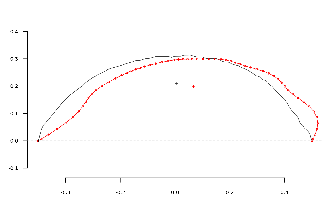
o <- olea[1]
o <- coo_bookstein(o)
coo_plot(o)
o.dfourier <- dfourier(o, nb.h=12)
o.dfourier
#> $an
#>  [1] -3.11820730 -0.13206715 -0.24781390 -0.09660325 -0.06788311 -0.06691169
#>  [7] -0.03519719 -0.06016120 -0.02071002 -0.06544994 -0.01169704 -0.06810722
#> 
#> $bn
#>  [1]  0.032926049 -0.914830858  0.005334948 -0.268975696 -0.006644877
#>  [6] -0.101625518  0.003834764 -0.049467452  0.003042230 -0.028964333
#> [11] -0.002260202 -0.022833346
#> 
#> $mod
#>  [1] 3.11838113 0.92431446 0.24787132 0.28579733 0.06820756 0.12167547
#>  [7] 0.03540548 0.07788709 0.02093227 0.07157253 0.01191341 0.07183283
#> 
#> $phi
#>  [1]  3.131034 -1.714168  3.120068 -1.915601 -3.044016 -2.153064  3.033070
#>  [8] -2.453432  2.995739 -2.724958 -2.950716 -2.818113
#> 
o.i <- dfourier_i(o.dfourier)
o.i <- coo_bookstein(o.i)
coo_draw(o.i, border='red')


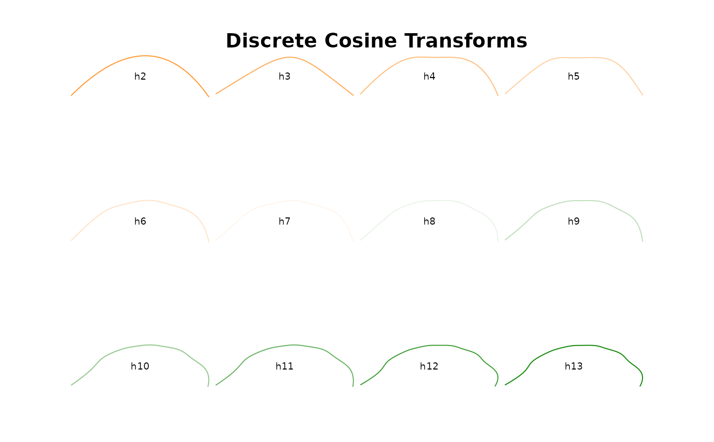
o <- olea[1]
h.range <- 2:13
coo <- list()
for (i in seq(along=h.range)){
coo[[i]] <- dfourier_i(dfourier(o, nb.h=h.range[i]))}
names(coo) <- paste0('h', h.range)
panel(Opn(coo), borders=col_india(12), names=TRUE)
title('Discrete Cosine Transforms')