Radii variation Fourier transform (equally spaced radii)

rfourier computes radii variation Fourier analysis from a matrix or a list of coordinates where points are equally spaced radii.

Usage

rfourier(x, ...)

# S3 method for default
rfourier(x, nb.h, smooth.it = 0, norm = FALSE, ...)

# S3 method for Out
rfourier(x, nb.h = 40, smooth.it = 0, norm = TRUE, thres = pi/90, ...)

# S3 method for list
rfourier(x, ...)

Arguments

x: A list or matrix of coordinates or an Out object
...: useless here
nb.h: integer. The number of harmonics to use. If missing, 12 is used on shapes; 99 percent of harmonic power on Out objects, both with messages.
smooth.it: integer. The number of smoothing iterations to perform.
norm: logical. Whether to scale the outlines so that the mean length of the radii used equals 1.
thres: numeric a tolerance to feed is_equallyspacedradii

Value

A list with following components:

an vector of \(a_{1->n}\) harmonic coefficients
bn vector of \(b_{1->n}\) harmonic coefficients
ao ao harmonic coefficient.
r vector of radii lengths.

Details

see the JSS paper for the maths behind. The methods for Out objects tests if coordinates have equally spaced radii using is_equallyspacedradii. A message is printed if this is not the case.

Note

Silent message and progress bars (if any) with options("verbose"=FALSE).

Directly borrowed for Claude (2008), and called fourier1 there.

References

Claude, J. (2008) Morphometrics with R, Use R! series, Springer 316 pp.

Examples

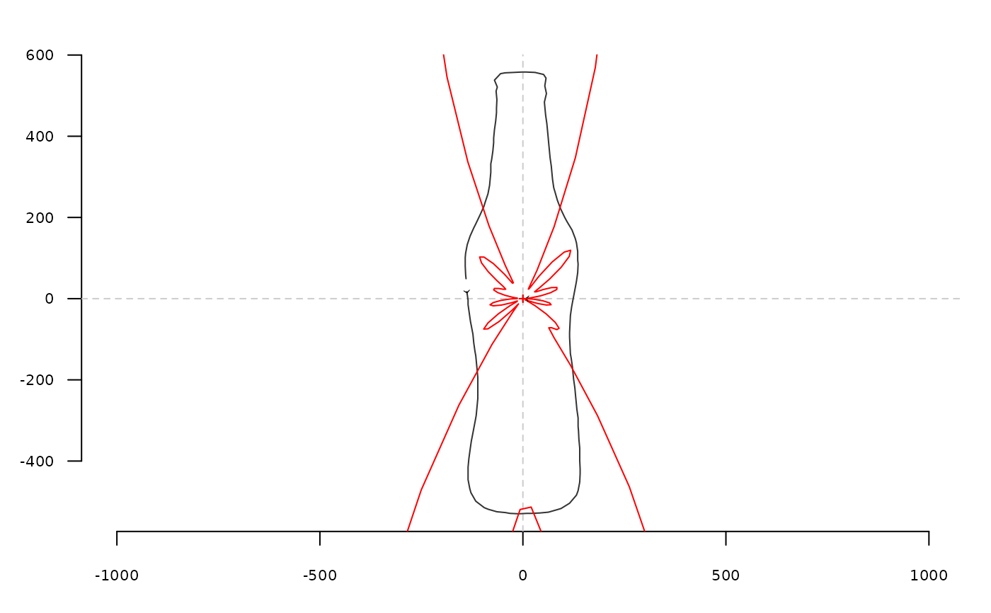
data(bot)
coo <- coo_center(bot[1]) # centering is almost mandatory for rfourier family
coo_plot(coo)
rf  <- rfourier(coo, 12)
rf
#> $an
#>  [1]  9.216460e-15 -4.745309e+02  8.327818e-01  2.719483e+02 -1.430955e+01
#>  [6] -1.110619e+02  2.489911e+01 -1.011701e+00 -1.771458e+01  5.542552e+01
#> [11]  6.786737e-01 -5.902187e+01
#> 
#> $bn
#>  [1]  1.054744e-13 -1.108663e+01 -5.032796e+01  1.187178e+01  1.332257e+02
#>  [6]  4.068663e+00 -1.709325e+02 -1.013725e+01  1.391797e+02  1.085760e+01
#> [11] -7.449979e+01 -2.355442e+00
#> 
#> $ao
#> [1] 669.1267
#> 
#> $r
#>   [1] 139.1167 135.1134 135.8741 136.8427 141.0323 143.5802 151.2095 162.8116
#>   [9] 175.5101 182.5204 198.0176 214.4721 223.4262 241.8735 260.7074 269.7883
#>  [17] 289.8301 310.0117 320.9760 342.0111 363.0862 373.1664 393.9569 415.7375
#>  [25] 436.2997 445.8192 465.8759 484.9159 494.7304 512.1917 523.5711 525.7951
#>  [33] 528.7641 528.6261 529.8403 529.9849 528.9630 529.2840 529.5332 529.6230
#>  [41] 526.6029 525.3373 516.8135 501.5361 492.0222 473.0432 453.3357 442.8940
#>  [49] 422.7064 402.9506 393.5883 373.2914 353.4743 342.9622 323.7894 303.5315
#>  [57] 283.8734 274.5648 254.3851 234.8608 225.9056 207.4851 188.9917 179.2651
#>  [65] 163.2102 148.4020 142.2876 131.8906 124.2115 121.7441 122.3408 126.4329
#>  [73] 133.8555 138.8126 149.4057 160.3977 165.1035 178.0327 190.2983 196.3891
#>  [81] 207.9233 218.2629 225.0539 239.8685 256.5975 274.7171 283.4915 303.0400
#>  [89] 323.0170 333.5460 353.5262 373.8148 383.4986 404.8965 425.3750 435.1409
#>  [97] 455.5781 476.1955 487.0166 508.4428 526.8989 546.1072 554.4755 557.9344
#> [105] 558.1869 558.1342 557.6074 557.8729 556.8590 542.6716 524.9317 515.3814
#> [113] 494.2988 473.6200 462.7267 442.2440 421.9866 401.6471 390.8306 370.6053
#> [121] 350.7010 341.4100 321.0176 301.2409 290.9421 272.0980 254.7364 246.6077
#> [129] 230.9259 217.6545 212.0765 201.6712 191.0722 180.1960 174.3784 163.0992
#> [137] 152.9502 148.4252
#> 
rfi <- rfourier_i(rf)
coo_draw(rfi, border='red', col=NA)


# Out method
bot %>% rfourier()
#> some shapes seem(s) to have some identical coordinates
#> 'nb.h' not provided and set to 60 (99% harmonic power)
#> An OutCoe object [ radii variation (equally spaced radii) analysis ]
#> --------------------
#>  - $coe: 40 outlines described, 60 harmonics
#> # A tibble: 40 × 2
#>   type   fake 
#>   <fct>  <fct>
#> 1 whisky a    
#> 2 whisky a    
#> 3 whisky a    
#> 4 whisky a    
#> 5 whisky a    
#> 6 whisky a    
#> # ℹ 34 more rows