Calibrate using reconstructed shapes

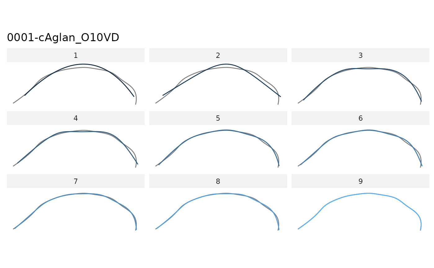
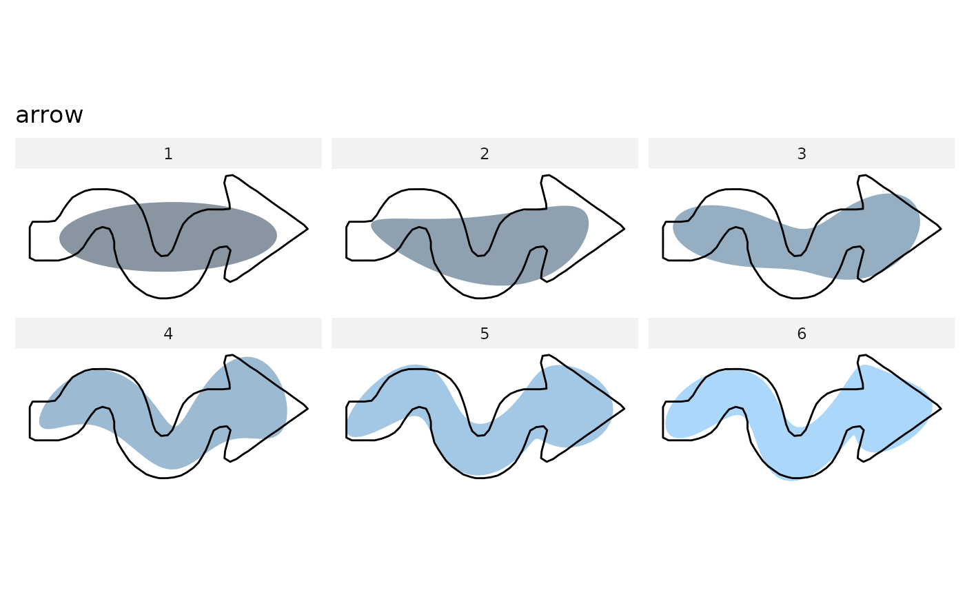
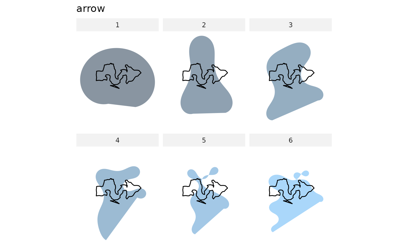
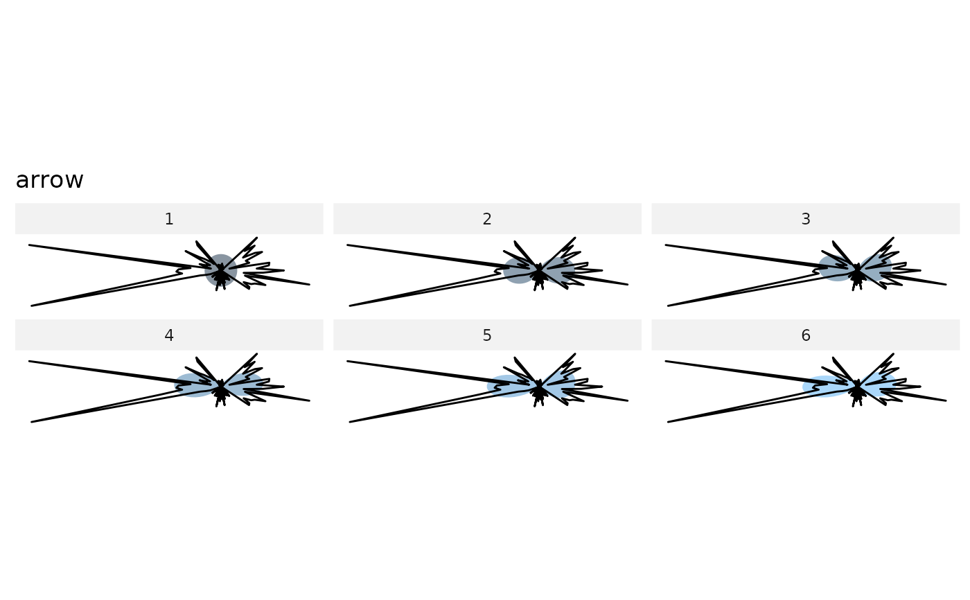
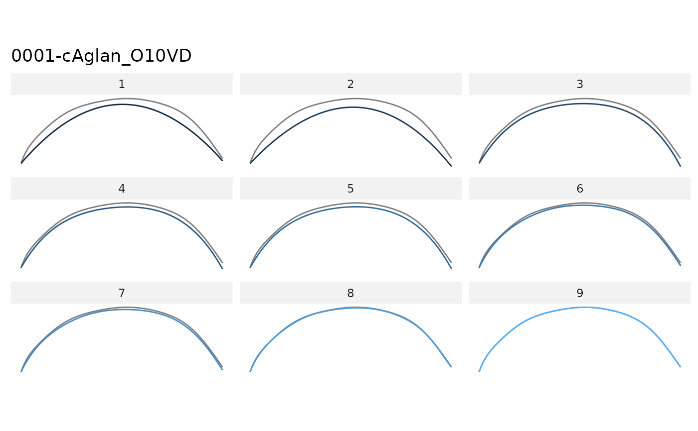
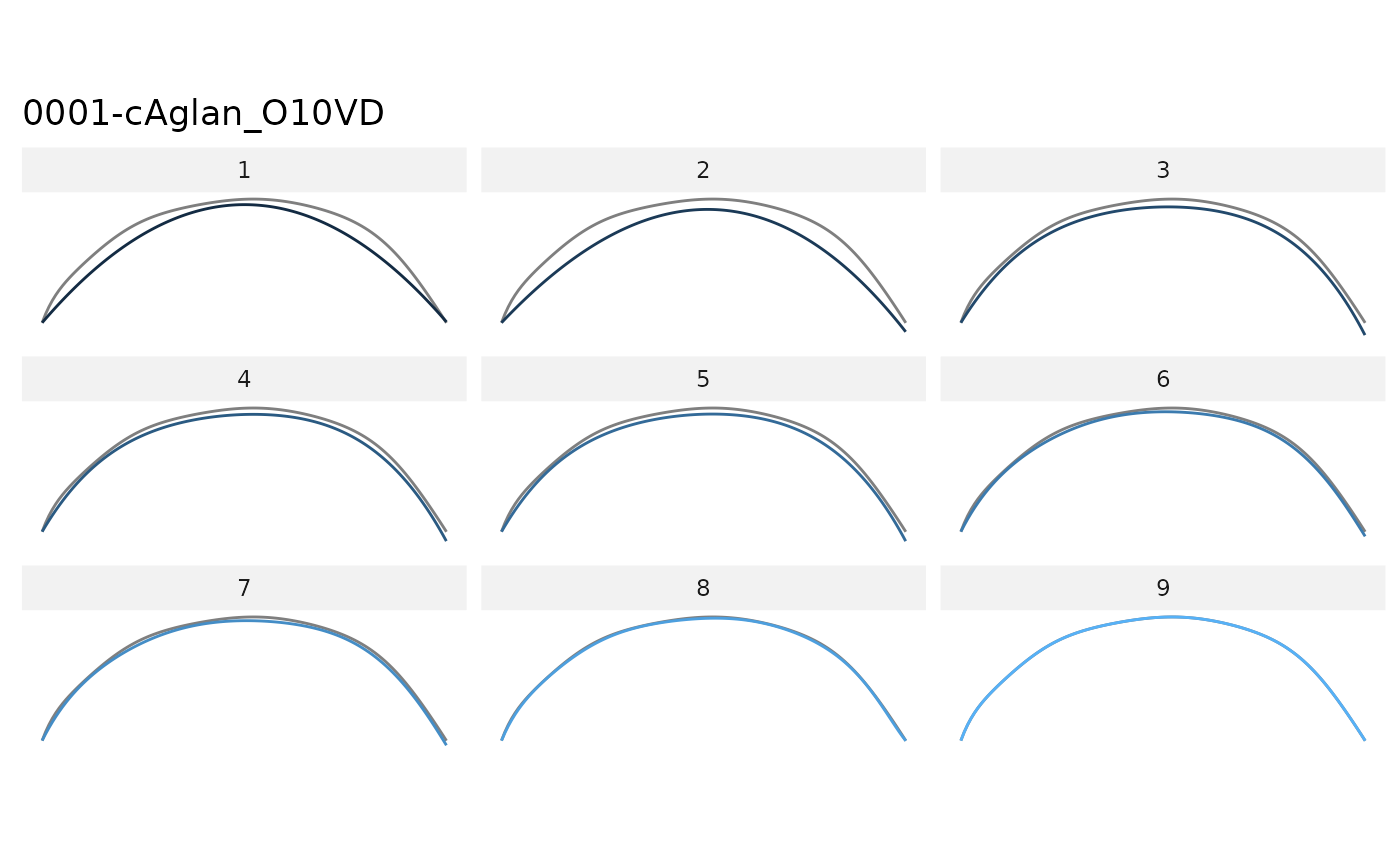
Calculate and displays reconstructed shapes using a range of harmonic number. Compare them visually with the maximal fit. This explicitely demonstrates how robust efourier is compared to tfourier and rfourier.

Usage

calibrate_reconstructions_efourier(x, id, range = 1:9)

calibrate_reconstructions_rfourier(x, id, range = 1:9)

calibrate_reconstructions_tfourier(x, id, range = 1:9)

calibrate_reconstructions_sfourier(x, id, range = 1:9)

calibrate_reconstructions_npoly(
  x,
  id,
  range = 2:10,
  baseline1 = c(-1, 0),
  baseline2 = c(1, 0)
)

calibrate_reconstructions_opoly(
  x,
  id,
  range = 2:10,
  baseline1 = c(-1, 0),
  baseline2 = c(1, 0)
)

calibrate_reconstructions_dfourier(
  x,
  id,
  range = 2:10,
  baseline1 = c(-1, 0),
  baseline2 = c(1, 0)
)

Arguments

x

the Coo object on which to calibrate_reconstructions

id

the shape on which to perform calibrate_reconstructions

range

vector of harmonics on which to perform calibrate_reconstructions

baseline1

\((x; y)\) coordinates for the first point of the baseline

baseline2

\((x; y)\) coordinates for the second point of the baseline

Value

a ggplot object and the full list of intermediate results. See examples.

See also

Other calibration: calibrate_deviations(), calibrate_harmonicpower(), calibrate_r2()

Examples

### On Out
shapes %>%
    calibrate_reconstructions_efourier(id=1, range=1:6)


# you may prefer efourier...
shapes %>%
    calibrate_reconstructions_tfourier(id=1, range=1:6)


#' you may prefer efourier...
shapes %>%
    calibrate_reconstructions_rfourier(id=1, range=1:6)


#' you may prefer efourier... # todo
#shapes %>%
#     calibrate_reconstructions_sfourier(id=5, range=1:6)

### On Opn
olea %>%
    calibrate_reconstructions_opoly(id=1)


olea %>%
    calibrate_reconstructions_npoly(id=1)


olea %>%
    calibrate_reconstructions_dfourier(id=1)